Entering data in Excel is the same as typing text and numbers into the cells in an Excel worksheet. Formatting data in Excel is a process of modifying and customizing the texts and numbers entered.
As discussed in Microsoft Excel Tutorial 1, a cell is an intersection between a column label and a row number. This box has a reference or an address that is referred to when performing computations and analysis.
Before we can analyze or compute data in MS Excel, we must first enter the necessary data row-wise or column-wise. Depending on the nature of the analysis, formatting data and cells may be necessary.
In this tutorial, we shall look at how to enter and format data in an excel worksheet.
Entering Data in Excel
Entering data in Microsoft Excel can be done in three major ways:
- By typing in data into individual cells in an Excel worksheet,
- By copying and pasting data from another source to selected cells in a worksheet
- By importing data from an external data source
Enter data in a row or column
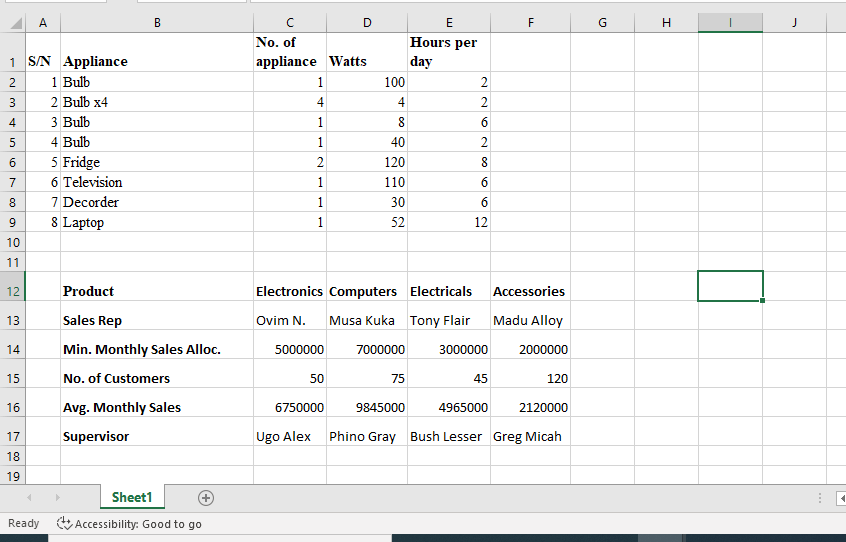
Microsoft Excel workspace, otherwise called worksheet is organized in columns and rows. To enter data by typing, you can arrange your data in a row or a column as shown below.
Then, you start typing on the first cell and arrange your column headings on the first row. Continue entering data on the cells below each column heading as you wish until you are done.
How you enter your data depends on the nature and purpose of the data. For more information on data entry in Excel, visit this post: Data Entry in Excel.
Using the fill command
When entering values in Microsoft Excel, you can fill in similar values and formulas across selected rows or columns automatically. This will save you the time and stress of typing similar data into the appropriate cells.
This fill command can be used manually or automatically. To use the manual fill command, do the following:
- Enter the data or formula in the first cell in a column or row.
- If it is a constant, e.g., 15, …, enter 15 in the first cell in a column or row.
- If it is a series, e.g., 1,2,…, enter the first two values in adjacent cells.
- Highlight the cell(s) with the values.
- You will see a small box in the bottom right of the highlighted cell(s).
- Click and drag the box downwards or rightwards to fill in values across columns or rows.
If you find it difficult to use this method, you can use the fill command on the Editing group as follow:
- Type the first value in a selected cell, and select that cell
- If you want to fill the same value across columns or rows, then, highlight a range of cells
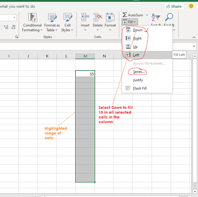
- On the Home tab, under Editing group, select Fill.
- From the fill dropdown menu, select any of Down, Right, Up, or Left.
- If you want to fill series of values different from each other, thenuse the Series dialog box.
- On the Fill dropdownmenu, select Series, a dialog box will appear.
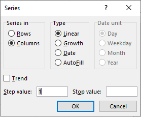
- On the dialog box, select Rows or Columns to specify where the values will fill across.
- Select Linear under Type and indicate a step and a stop value. You can choose any other type (growth, date, etc.) depending on your need.
- Click Ok, when you are done. The selected series will be filled automatically across the selected cells.
Copy and paste data in selected cells
You can also enter data in Microsoft Excel by copying from another source and pasting it in a worksheet. This method can be easily achieved by using the clipboard. See how to use the clipboard in our post on: Inserting and Formatting Texts.
To copy and paste data in Excel, do the following:
- Locate the source of the data.
- When the data source is opened, select the required data and press CTRL+C on the keyboard.
- Open the worksheet where you want to paste the data.
- Select a cell in the worksheet. The selected cell will mark the starting location to paste the data.
- If you want the data to be placed in a particular range, then select the range.
- On the Home tab, under the Clipboard group, click Paste. You can also press the CTRL+V key on the Keyboard.
The paste special command
Microsoft Excel gives you different paste options called paste special. When you copy or cut an item in Excel, you have the option to choose from different paste types.
There are about 14 different options namely:
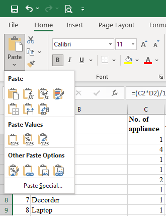
- Paste: This option is used to paste the copied item(s) using default settings.
- Paste formula: This option is used to paste formulas in selected cells
- Paste formula and number formatting: This is used to paste formula and inherent number formatting on the copied data.
- Keep source format: This is used to paste an item including all formats on the copied data.
- No borders: Used when a copied data has borders. Use this option to remove the borders.
- Keep column width: This is used to maintain the column width of the source data.
- Paste transpose: This is used to paste copied items, and transpose them from column to row and vice versa.
- Paste values: this option will remove all formulas and formatting on the copied items and paste only values.
- Values and number formatting: here, you will keep values and number formatting only.
- Values and source formatting: Here you will keep values and source formatting only
- Paste formatting: paste only the cell formatting of a copied item
- Paste link only: paste the link address of a copied item
- Paste picture: paste copied items as a picture
- Paste copied items as a picture with the link
- If you choose the Paste Special… option, a dialog box will appear. On the dialog box, select your required options and click OK.
Undo and redo
When entering and formatting data in Excel and other applications, you may need to undo or redo what was done. The undo and redo commands are located on the QA toolbar.

The undo command is used to revert from current editing to the previous editing in the undo history. While the redo command is used to revert from the previous editing to the current editing.
For example, if I type 15 in a cell and delete it, and replacing the value with 20. I can revert to 15 by clicking the undo button or CTRL+Z on the keyboard. Similarly, if I want to go back to 20, I will click the redo button or CTRL+Y on the keyboard.
The undo and redo command usually keep track of editing done in a workbook in a history log. To go deeper in the log, click the dropdown arrow button and select the entry you want to undo.
Importing data into Excel
The third way you can enter data into excel is by importing data from an external source. Excel gives us the option of importing data from different data sources including a database, text file, webpage, etc.
To import data from an external source, do the following: (We shall import data from a text file).
- Open an Excel workbook with a blank worksheet. You can also select an empty cell in an existing workbook.
- On the Data tab, click on Get External Data. From themenu that appears, select your source of data. (NB: The data must be available in the selected format). In our case, choose From Text.
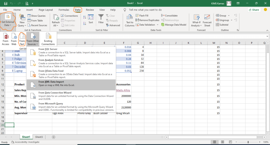
- The Import text file dialog box will appear.
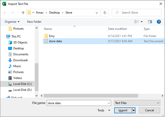
- On the dialog box, locate and select the appropriate file you want to import its data and click Import.
- The Text Import Wizard window will appear.
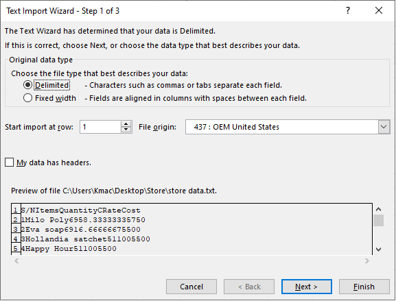
- On the text import wizard window, choose the Delimited or Fixed width option. This depends on how your data is typed. In this example, we choose the Delimited.
- Select My data has headers (if your data has headers: see the preview) and click Next.
- On the next page, choose your type of delimiter, e.g. tab, comma, etc. Click Next to continue.
- On the last page, choose the General Column Data Format.
- When done, click Finish.
- A dialog box appears requesting how and where to place the data in your worksheet.
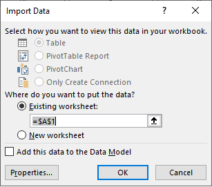
- On the dialog box, select any of Table, PivotTable Report, etc.
- Also, select the location for the data. If you choose an existing worksheet, select a cell address. You can leave the default.
- Click Ok and wait for Excel to import the data.
- NOTE: If you want to import data from an existing table in your workbook, select Existing Connection. From the dialog box that appears, select the Tables tab, then the table and click open. Then continue from 11 above.
These are the three (3) basic methods you can use to enter data into Microsoft Excel and other spreadsheet apps.
Formatting data in Excel
Formatting data in Excel involves modifying texts and numbers entered in cells to carry out an analysis. Data entered in Excel may be for presentation, computation, or analysis purposes.
Alignment
Like in Microsoft Word, three types of alignment exist in Microsoft Excel. They include the left, center, and right alignments. Because data is stored in cells, each of these basic alignment types has three modifications: top, middle and bottom.

This means that you can align data in any of the nine different ways: top-left, middle right, bottom center, etc.
When a text is entered, it is aligned at the bottom-left by default, while a number is aligned at the bottom-right by default.
To change the alignment of data in cells, do the following:
- Select the cell or range of cells to be aligned
- On the Home tab, under the Alignment group, select any of the alignment types you want.
- The selected alignment will be applied automatically on the selected cells.
Text and number formatting
You can perform text and number formatting in Excel just as you will do in a Microsoft Word document.
The difference is that instead of selecting text as in word, you will select cells in Excel. The values in cells take the formatting of the cells they reside.
To format the cell content,
- Select the cell or range of cells you want to apply formatting on.
- On the Home tab, under the Fonts group, locate and select the formatting command you want.
- Select your desired command, the content will be automatically formatted. For detail, see Inserting and Formatting Texts.
Formatting cells in Excel
When entering data in excel, other forms of alignment could be used. These types of formatting affect the selected cells and their content. They include merging, shrinking, and wrapping cells.
Merge cells
Merging cells means combining more than one cell. When more than one cell is merged, the combined cells become one. All cells in the group retain the address of the first cell in that group.
If there is content in the cells before the merging, the content of all the cells is lost. However, the content of the first cell in the group is retained. It becomes the content of the merged cell.
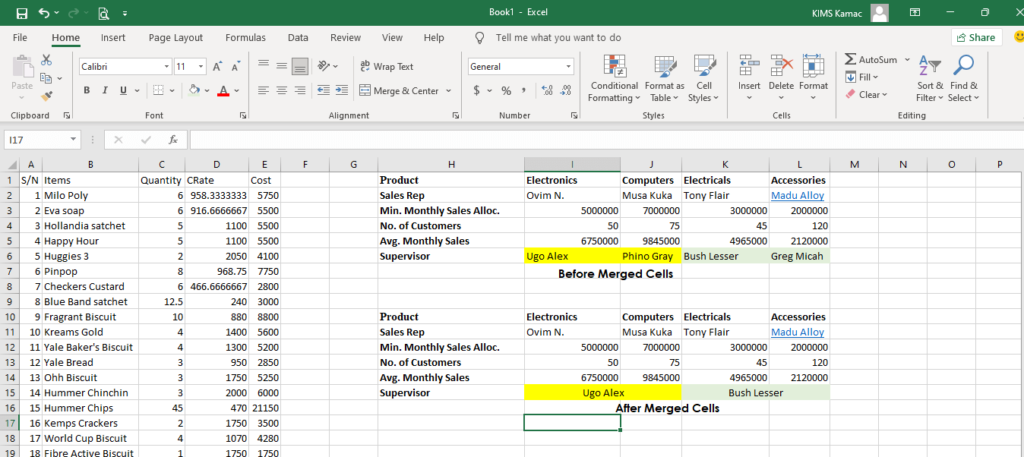
To merge cells, do the following:
- Select the group of adjacent cells you want to merge
- On the Home tab, under Alignment group, select Merge & Center.
- The selected cells will be automatically merged.
- Other options exist when you click the dropdown arrow on the Merge & Center command. Experiment with them.
- To unmerge cells, select the merged cell
- On the Home tab, under Alignment group, select Merge & Center. You can click the dropdown arrow button and select Unmerge Cells from the list
Shrink cell content
You can use shrink to fit to reduce the size of the content in a cell. When this is done, the content fits inside the cell without requiring adjustments. However, this is not good when the content is too big for a cell. It can be used only when the content exceeds the size of the cell a little.
To apply shrink to fit, do the following:
- Select the cell or group of cells you want to shrink its content.
- On the Home tab, under Alignment group, select Alignment dialog box launcher.
- A dialog box appears.
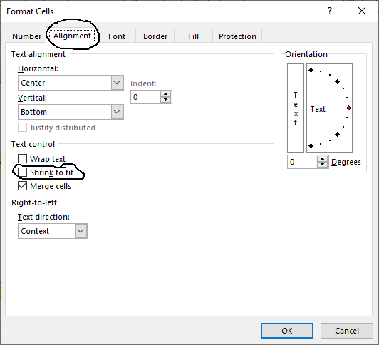
- In the dialog box, under the Alignment tab, select the Shrink to fit option button.
- Click Ok when done. The content of the selected cells shrinks to enter the cell.
Wrap cells
Wrapping is used to create a multiline text in a worksheet cell. When the content of a cell is too big, you can either expand the column or wrap the content. If none of this is done, the data in the cell will not show clearly.
To wrap the content of a cell, do the following:
- Select the cell or group of cells you want to wrap their contents
- On the Home tab, under the Alignment group, select Wrap Text.
- The content of selected cells will be automatically wrapped.
- To unwrap the cells, select the wrapped cell and click on the Wrap Text command icon.
Conclusion
We have come to the end of today’s Microsoft Excel tutorial. We were able to look at entering and formatting data in Excel. We began by discussing how you can insert data in a workbook.
We looked at three basic ways of entering data in a worksheet to include: typing, copying, and importing data.
We further discussed how to format data in Excel. We discovered that formatting data in excel implies formatting cells in Excel. This is because data assumes the formatting of the cells they reside. We concluded by looking at different cell formatting options including alignment, merging, and wrapping the content of cells.
These are the basics you need to know before we go into computing and analyzing data in Excel. Particularly, we shall discuss conditional formatting in Excel.


