A worksheet in Excel is a collection of cells organized in columns and rows as in a table. A worksheet is a workspace where a user enters data and performs the necessary computations on data.

Worksheet in Excel 2016, is made up of 16384 columns and 1048576 rows with columns labeled from A to XFD.

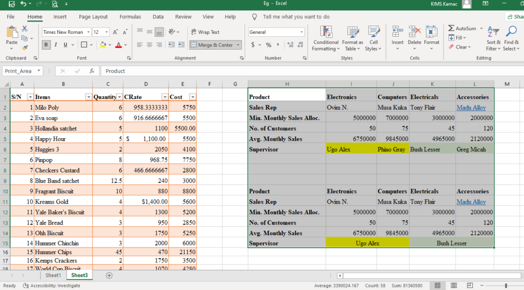
Due to the size of an Excel worksheet, it is difficult to use all the cells in a worksheet. However, you can format data, convert a range to a table, print a range and entire worksheet. For example, the worksheet below displays data with different formatting, and a selection to be printed.

By default, Excel 2016 has one worksheet. You can add more sheets in a workbook, but one worksheet will always be active at a time. Protecting a worksheet restricts users from modifying its content.

When numeric data is entered in a worksheet, you can format them using available number formats. In this tutorial, we shall discuss how to format numbers and manage worksheets in excel.

Formatting numbers in Excel

When you enter numeric data in an Excel worksheet, you have the liberty to format the cells. There are different number formats you can use when formatting numbers in excel. Some of them include currency, percentages, decimals, dates, and phone numbers.

Number formats

There are 12 number formatting commands in Excel that you can use to format your cells in a worksheet. They include the following:

General: This is the default number format that Excel applies to every data entered in a worksheet, except explicitly specified.
Number: When formatting numbers you can use the number format to indicate a number. If this format is used, you can use a thousand separators and specify the number of decimal places.
Accounting: When used, it displays the currency symbol, a thousand separator, and rounds to 2 decimal places. However, it aligns the currency symbol to the left.
Currency: When used, it displays the currency symbol, a thousand separator, and rounds to 2 decimal places. However, it aligns the currency symbol with the number.
Percentage %: used to multiply a number by 100, and attaching the % sign.
Fraction: Used to display a fractional number.
Scientific: Is used to display a number in exponential notation thus, AE+n. For example, 6580025864 can be displayed as 6.58E+9.
Date: used to format date values of different formats.
Time: used to format time values.
Text: Converts content to text even if it is a number value. Values with the text number format cannot be used for computations.
Special: used to display numbers as zip code, and phone number. Formats are usually displayed in United States patterns.
Custom: Used to modify a number format. You can use it to add a number format of your choice. For detail about custom number formats, visit here.

Apply a number format to a cell

Select a cell or range of cell
On the Home tab, under the Number group, select the dropdown arrow.

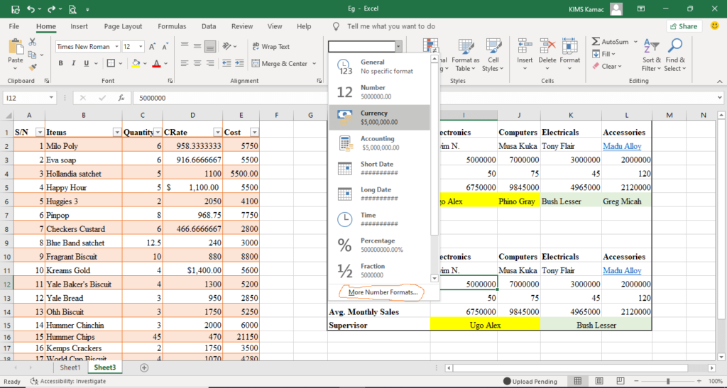
Select any of the number formats from the list
It will be applied automatically to the selected cell or range.

You can also, apply formatting to numbers by invoking the number dialog box. To open the dialog box, do any of the following:

Press CTRL+1 on the keyboard, and select the Number tab.
Click the number dialog box launcher on the Number group.
From the dropdown list on the Number group, select More Number Formats…
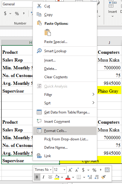
Right-click a cell or range of cells and select Format Cells… from the popup list

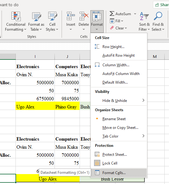
On the Home tab, under Cells, select Format. From the dropdown list, select Format Cells…

When the dialog box appears, select the Number tab.

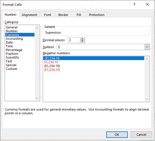
On the dialog box, choose a number format and the necessary features you want.
When done, click OK.

Managing worksheets in Excel

Managing worksheet in Excel includes modifying worksheets for ease of use and access. You can insert, rename, copy or delete a worksheet in excel.

Insert a Worksheet

Microsoft Excel 2016 has one worksheet by default. To include more than one worksheet in a workbook, you will need to insert more sheets. To insert a worksheet, do any of the following:

On the base of the Sheet, select the (+) icon to the right of the last sheet in a workbook.
On the Home tab, under Cells, select Insert. From the list, select Insert Sheet.
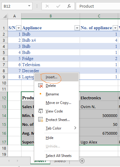
Right-click an existing worksheet. From the popup list, select Insert. Select Worksheet on the dialog box that appears, and click OK.

Rename a worksheet

To rename a worksheet, do any of the following:

Double-click the sheet you want to rename. When the name is selected, delete the existing name and type a name of your choice.
Right-click the sheet you want to rename. Select Rename from the popup list. Rename the selected sheet.

Delete a worksheet

To delete a worksheet, do any of the following:

Right-click the sheet you want to delete. Select Delete from the popup list. Select Delete from the dialog box that appears.

On the Home tab, under Cells, select Delete. From the list, select Delete Sheet.

NB: If the sheet you are deleting does not have content, the sheet will be deleted outrightly. If the sheet has content, a dialog box will notify you that all the content will be permanently deleted.

Move or copy a worksheet

To move a worksheet, select and drag the worksheet tab to any tab location of your choice.

To copy a worksheet, do the following:

Hold the CTRL key and drag the worksheet tab to a tab location of your choice.
Right-click the worksheet you want to copy.
1. From the popup list that appears, select Move or copy

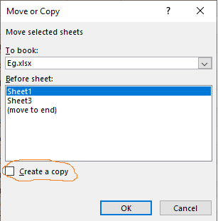
From the dialog box that appears, select the Create a copy check box
- Under Before sheet, select where you want to place the copy of the sheet.
- Click OK when done.

Hide/unhide a worksheet

If you want to hide a worksheet, do any of the following:

Right-click the sheet you want to hide, and select Hide from the popup list. The sheet will be automatically hidden.
On the Home tab, under the Cells group, select Format

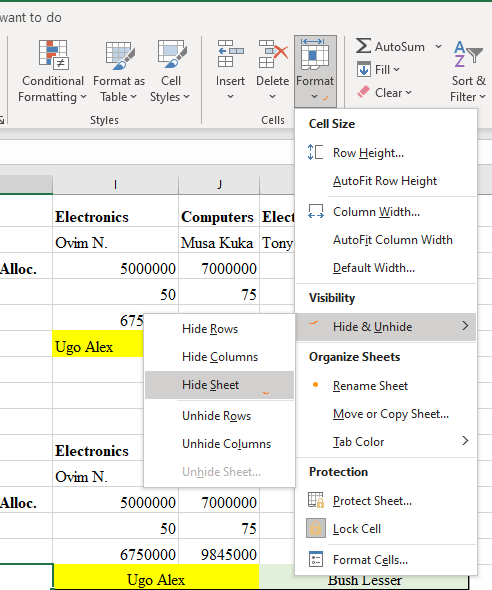
From the format dropdown list, point to Hide & Unhide and select Hide Sheet.
The selected sheet will be hidden.

To unhide a worksheet, do the following:

Right-click any worksheet tab, and select Unhide from the popup list.
On the Home tab, under the Cells group, select Format.
- From the format dropdown list, point to Hide & Unhide and select Unhide Sheet.
In either case, a dialog box will appear.

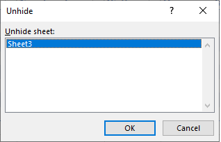
On the dialog box, select the sheet you want to unhide and click OK.
The selected worksheet will appear.

Grouping Worksheets in Excel

When you need to perform the same action in more than one worksheet, it’s easier to group them. Grouped worksheets make it easier to enter the same data in more than one worksheet at the same time.

For example, you can do any of the following, and more in a grouped worksheet.

Enter the same data/ formula/ formatting in more than one worksheet at the same time
Perform the same calculation in more than one worksheet
Move, copy or delete more than one worksheet
Print selected worksheets
Correct similar typographic error in more than one worksheet

Grouping worksheets will help you save time and eliminate redundant data entry.

Group worksheets together

To group a worksheet, the worksheets should have similar structures. Do the following to group worksheets:

Press and hold the CTRL key on the keyboard, and select the worksheets you want to group together
If the sheets are together, then, select the first sheet, hold the SHIFT key, and select the last sheet.
Start modifying the worksheets.

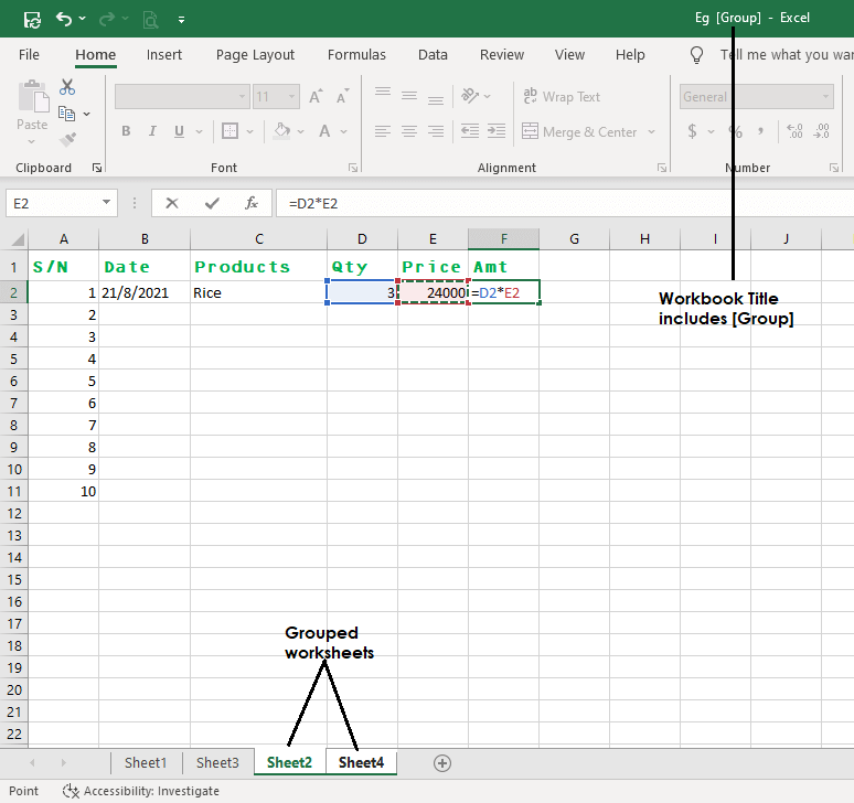
All changes will take place in all grouped worksheets at the same time.

Move or copy a grouped worksheet

You can move a grouped worksheet by:

Clicking on a tab on the grouped worksheet
Drag the group to any tab location of your choice

To copy grouped worksheets:

Right-click any of the grouped worksheets you want to copy.
From the popup list that appears, select Move or Copy
From the dialog box that appears, select the Create a copy check box
Under Before sheet, select where you want to place the copy of the grouped worksheets.
Click OK when done.
The sheets are automatically copied to the chosen location.

Ungroup selected worksheets

To ungroup selected worksheets:

Hold the CTRL key and select the sheet you want to ungroup.
To ungroup all grouped sheets, simply click on one of the sheets that are not grouped.

Group all worksheets in a workbook

Right-click on one of the sheets tab.
From the popup list, select Select All Sheets
NB: When you group all worksheets, you can ungroup them by clicking on any of the sheets’ tabs. Hence, you cannot browse through the sheets when you grouped all worksheets. However, you can browse through grouped worksheets, if all sheets in a workbook are not grouped.
Youcan also ungroup all worksheets by right-clicking a sheet, from the popup list, select Ungroup Sheets.

Deleting a grouped worksheet

Right-click the grouped worksheet you want to delete. Select Delete from the popup list. Select Delete from the dialog box that appears.
On the Home tab, under Cells, select Delete. From the list, select Delete Sheet.

Hiding grouped worksheets

If you want to hide a grouped worksheet, do any of the following:

Right-click the grouped sheet you want to hide, and select Hide from the popup list. The grouped worksheets will be automatically hidden.
On the Home tab, under the Cells group, select Format
- From the format dropdown list, point to Hide & Unhide and select Hide Sheet.
- The selected sheets will be hidden.

Unhiding grouped worksheets

To unhide hidden grouped worksheets, do the following:

Right-click any worksheet tab, and select Unhide from the popup list.
On the Home tab, under the Cells group, select Format.
- From the format dropdown list, point to Hide & Unhide and select Unhide Sheet.
In either case, a dialog box will appear.
On the dialog box, select the sheet you want to unhide and click OK.
Repeat the same process until you are done.

Modifying Columns and Rows in Excel

As earlier discussed, the worksheet in Excel is made up of rows and columns. Columns are vertical cells that run from up to down. They have a column label that begins with A and ends in XFD.

Similarly, rows are horizontal cells that run from left to right. They have row numbers that begin with 1 and end in 1048576.

Both columns and rows play an important role in a worksheet because their combination gives birth to a cell. Also, the column label and row number are used as a reference or an address for every selected cell.

When working on a worksheet, there are columns and rows modifications that are necessary for effective management. In this section, we shall discuss how to insert, delete, hide and resize columns and rows in Excel.

Inserting and Deleting Columns and Rows

Assuming you are working on a worksheet, and there is a need for you to add a column or row. For example, in the worksheet below, I want to add a column before Watts and a row before Fridge.

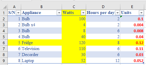
To achieve this, do the following:

To insert a column:

On the worksheet, select a cell on column C or the entire C column.
On the Home tab, under the Cells group, select Insert.
From the dropdown menu, select Insert Sheet Columns.
The column will be added, shifting the Watts column to the right. Hence, the new column becomes column C.
You can also, right-click on top of the Column C label. From the popup list, select Insert.

To Insert a row:

On the worksheet, select a cell on row 6 or the entire Row 6.
On the Home tab, under the Cells group, select Insert.
From the dropdown menu, select Insert Sheet Rows.
The row will be added, shifting Fridge Row down. Hence, the new row becomes row 6.
You can also, right-click on the row number “6”. From the popup list, select Insert.

The output of the above exercise is shown in the image below.

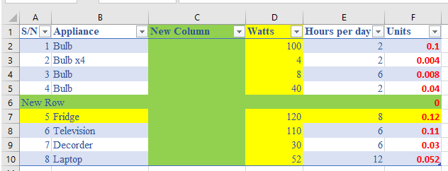
To delete a column/ row,

On the worksheet, select the columns or rows you want to delete or a range within the columns/ rows
Go to Home, under Cells, select Delete
From the dropdown menu that appears, select either Delete Sheet Columns or Delete Sheet Rows
The columns or rows will be automatically deleted.

Inserting Multiple Columns & Rows

To insert more than one column or row in a worksheet, do the following.

For columns:

Highlight the number of columns you want to insert beginning from the insertion point, e.g., 4 columns
Hold down the SHIFT or CTRL key on the keyboard.
With the CTRL or SHIFT pressed, right-click one of the selected column labels
From the dropdown menu, select Insert.
The exact number of highlighted columns will be inserted, moving other columns to the right.

For rows:

Highlight the number of rows you want to insert beginning from the insertion point, e.g., 3 rows
Hold down the SHIFT or CTRL key on the keyboard.
With the CTRL or SHIFT pressed, right-click one of the selected row numbers
From the dropdown menu, select Insert.
The exact number of highlighted rows will be inserted, moving other rows down.

TIP: If the selected column or row has formatting applied, the new column/ row will inherit the formatting. To remove the formatting, select the Insert Options button on the inserted column/ row, and select Clear Formatting.

Inserting & Deleting Cells

To insert cells,

Select the cell or range where you want to insert cell(s)
Right-click the selected cell(s), from the popup menu, select Insert
A dialog box appears

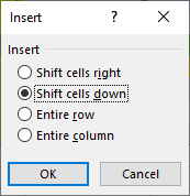
On the dialog box, choose either Shift cells right or Shift cells down.
You can also go to Home > Cells > Insert > Insert Cells...

To Delete a cell,

Select the cell or range you want to delete
Right-click the selected cell(s), from the popup menu, select Delete
A dialog box appears
On the dialog box, choose either Shift cells left or Shift cells up.
You can also go to Home > Cells > Delete > Delete Cells...

Modifying cell width and height

To adjust column width,

Place the pointer on the line that divides two columns, the pointer changes to a cross.
Click and drag to the left (to reduce width) or to the right (to expand width)

You can also, adjust more than one column at the same time and with equal width by,

Select the cell, or range, or columns you want to adjust their width
Go to Home, under Cells, select Format
From the format, cells drop-down menu, select Column Width…

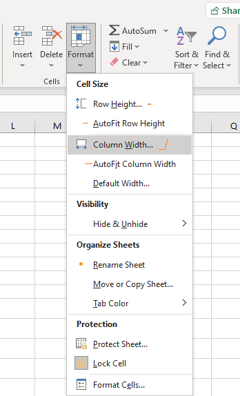
resize multiple columns/ rows at the same time

A dialog box appears, enter a width size, and press OK.
You can also choose AutoFit Column Width to fit columns according to the content width.

To adjust row height,

Place the pointer on the line that divides the two-row numbers, the pointer changes to a cross.
Click and drag to up (to reduce height) or to down (to expand height)

You can also, adjust more than one row at the same time and with equal height by,

Select the cell, or range, or rows you want to adjust their height
Go to Home, under Cells, select Format
From the format, cells drop-down menu, select Row Height…
A dialog box appears, enter a height size, and press OK.

Hiding and Unhiding Rows and Columns

If you want to hide a column or row, do the following:

To hide column/ row

Highlight the columns/ rows you want to hide
Right-click the column label or row number, and select Hide from the popup list.

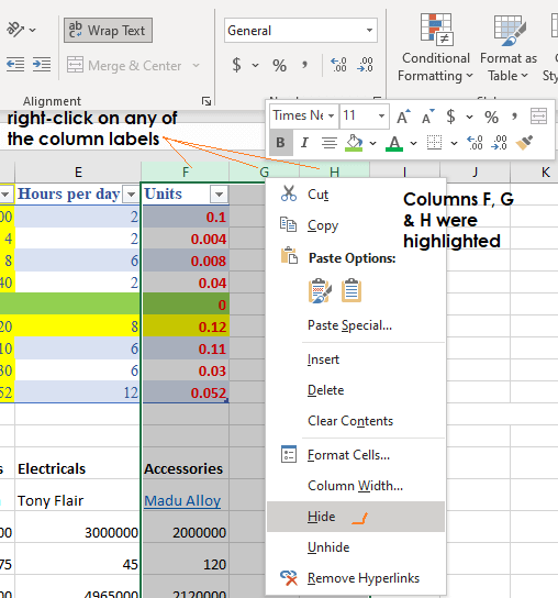
The sheet will be automatically hidden.
OR, On the Home tab, under the Cells group, select Format
- From the format dropdown list, point to Hide & Unhide and select either Hide Rows or Hide Columns.
- The selected column/ row will be hidden.

To unhide column/ row:

When you hide a column or a row, a double line appears where there is a hidden column/ row.

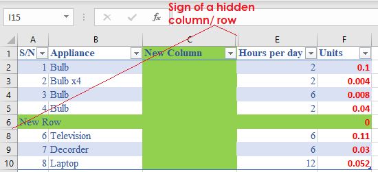
To unhide a column/ row do any of the following:

If only one column/ row was hidden, then, place the pointer on the double line and double-click. The hidden column/row will appear.
If more than one column/ row is hidden,
- Select adjacent columns/ rows between the hidden columns/ rows
- On the Home tab, under the Cells group, select Format.
- From the format dropdown list, point to Hide & Unhide and select Unhide Columns or Unhide Rows
All hidden columns/ rows will appear.

Conclusion

Thank you for staying with me till the end of this tutorial. In case you have further questions please, contact us as soon as possible.

Today’s tutorial centered on working with a worksheet in Excel. We looked at formatting numbers, managing worksheets, and modifying rows and columns in Excel.

Please, do not forget to visit the previous tutorials in Microsoft Word and Excel, in case you missed them:

If this tutorial has helped you, kindly share it with friends and colleagues. Next week we shall look at What is cell referencing in Excel.

Blog

Formatting Numbers and Worksheet in Excel