Introduction
We have walked through the basics of the Microsoft Excel Spreadsheet application. The basic knowledge is not enough to work in some establishments such as telecommunications, oil and gas, manufacturing, and so on. We shall therefore undertake data entry in Microsoft Excel in this article.
To be well equipped, we need to finetune our basic knowledge and upgrade our skills to intermediate and advanced levels. This is what we shall be doing beginning from this week. We shall use life examples for a better understanding.
Please, feel free to ask questions in the comment box, no matter how trivial.
Data Entry in Microsoft Excel
Data in Microsoft Excel depends on what we want to achieve, our main objectives and purposes for which the data is meant. Hence, before we begin data entry, we should ask ourselves the following questions:
- What is the purpose of the data?
- Is it for presentation and printing only?
- Is it for analysis?
- If it is for analysis, what kind of analysis?
It is important that we understand that data can be entered in Microsoft Excel in different ways depending on the kind of analysis we want to perform. Take a look at the following example:

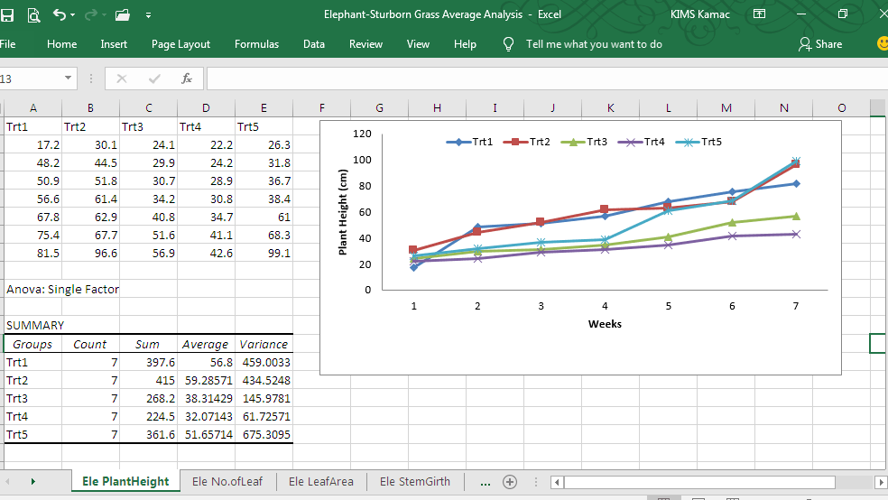
Data Entry For Analysis
The above image displays a simple data entry in Microsoft Excel, but it was used for the purpose of analysis.

Data Entry For Presentation and Printing
This second image shows yet a simple data entry in Microsoft Excel, but it was not meant for analysis, but for printing and presentation.
In addition to the above, we should have it in our mind that certain analysis does not permit some form of data entry. For example, when our purpose is to perform subtotal or pivot table analysis, we may not be permitted to use merged cells during data entry.
With the basic knowledge of Microsoft Excel already in our portfolio (if you are starting, please, go through Beginners Guide to Microsoft Excel Spreadsheet Application 1 and 2); from this week, our job is to walk you through various Microsoft Excel skills, including basic, intermediate and advanced skills to boost the requisite knowledge to work in any establishment.
Data Entry for Printing and Presentation
When entering data in Microsoft Excel for the sake of presentation and /or printing, our aim is to set up the page and ensure that data entered is presented on a page-wise basis. To do so, we should consider the following:
- Get the raw data on paper: It is important that the data to be entered in Microsoft Excel be first represented in a paper. This could be already existing data or currently observed data. The raw data will provide you with the information that will assist you on how to present the data in a spreadsheet.
- Setup the page: As soon as you have the data to be presented with you, it is now your duty to set up your page by adjusting the orientation, paper size, and margins of your pages.
- Use the page break preview: As you begin to enter your data, always switch between the normal view and page break view, if you are not using the page layout view. This will help you to keep your data within the page limits and ensure that there are no overlaps.
- Use page layout view: If your data requires that you create a repeated header in all the pages, including logo, then use the page layout view to ease your data entry.
- Start entering data: When you have finished setting up your pages, start entering the data as required. But pay attention to your data types.
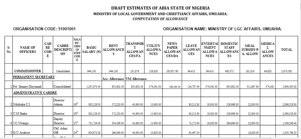
We are going to illustrate the above using two examples. In the first example, we shall create a Microsoft Excel worksheet that looks like this:
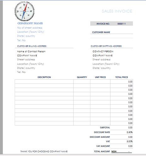
And in the second example, we shall produce a Microsoft Excel worksheet that looks like this:


In both cases, we shall visit some of the features we have introduced in our previous posts.
Simple Data Entry
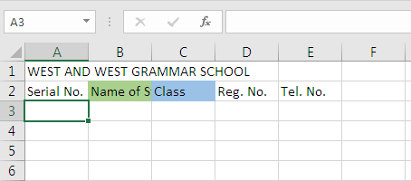
Entering data in Microsoft Excel is very simple. It entails you to type in the data in columns and rows, on a cell by cell basis; making sure that you did not skip a cell mistakenly. Let us illustrate this using students’ information in West and West Grammar School.
- Open Microsoft Excel workbook
- In the first cell (cell A1), type WEST AND WEST GRAMMAR SCHOOL
- In the second row and first column (cell A2) type Serial No, then, go ahead and type the following in row 2: Name of Student (cell B2), Class (cell C2), Reg. No. (Cell D2), and Tel. No. (cell E2).
- The result of (No. 3) above is shown below:

Note: The most common mistake I’ve seen people making while entering data is to jump a cell because the data in the previous cell covered the next cell. For example, when entering Name of Student, you will observe that it will overlap to cell C2, as shown below:


But this does not mean that cell C2 is occupied. Please, select cell C2 and type Class. always avoid this kind of mistake when entering data. If a cell is too small to contain the data in it, adjust the column width or row height, or use any of wrap text or merge cells commands (see Excel Basics).
- Adjust the cells as required and format the texts and complete the data entry, as shown below.
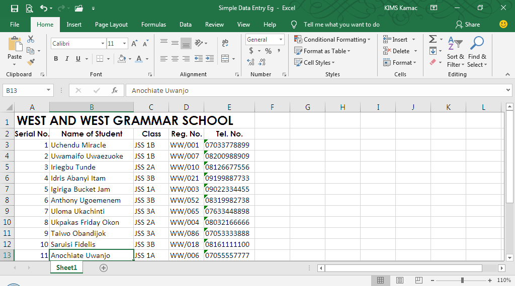

This is a very simple way to enter data in Excel.
Let us go to another example that is more complex, yet simple.
Data Entry for Presentation
In this example, we shall reproduce what looks like this:


This is a tabular work done in excel for presentation. A header is used to create the heading so that it will appear in all pages of the document, and all the data were fit in so that it can be printed in one page.
Let us start creating the table.
- Open an Microsoft Excel workbook and click the Page Layout view as shown below.


- In the add header area, type the document header. (Notice that the header area has left, center and right boxes). To centralize the header, type the heading in the center box. After you have typed the header, we have the following:
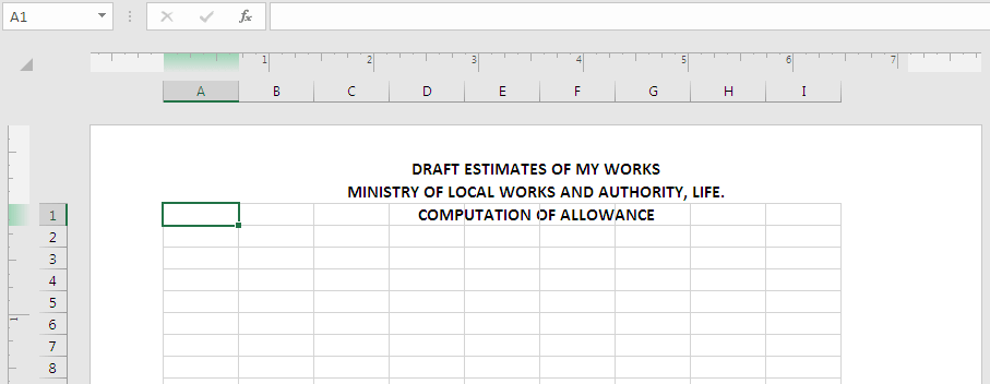

Note: A close look at the above shows that the last line of our header entered in the first row of our worksheet, also, the width of our page is smaller than what we want to type in the worksheet. Hence, we need to make some adjustments.
- Before we start typing, let us make the
following adjustments, change page orientation (to increase the width of the
page), change paper size (so our content can enter in the page), change the
margin (to push out the header from the first row).
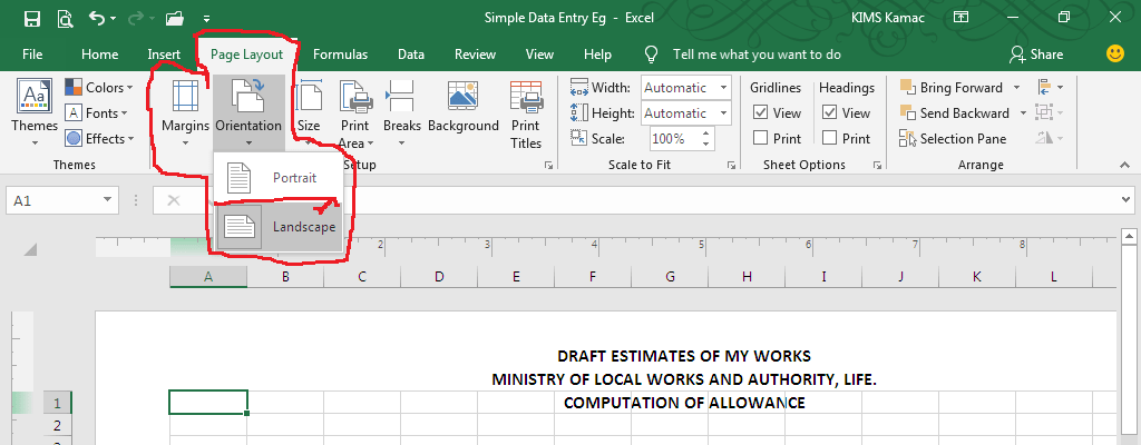
- Change page orientation: in the Page Layout tab, click on Orientation and select Landscape. See image below.

- Change paper size: in the Page Layout tab, click on Size and select Legal. See image below.


- Adjust margin: Here, we can adjust the top, bottom, right, and left margins. We will increase our top margin so as to push the header out of the row, then reduce our left and right margins, so we can have more room that will contain the data in a page. To adjust the margin, in the Page Layout tab, click on Margins and select Custom Margins, as shown.
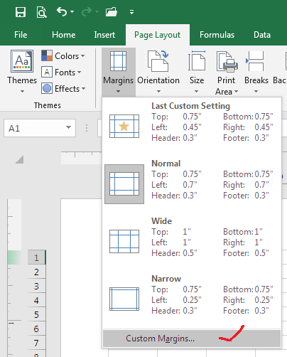

- In the Custom Margins dialog box, increase the top margin to 1pt, right, bottom and left margins to 0.45pt, then click OK.
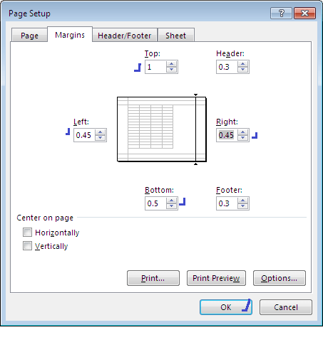

- If you do everything as specified above, your page will look like this:
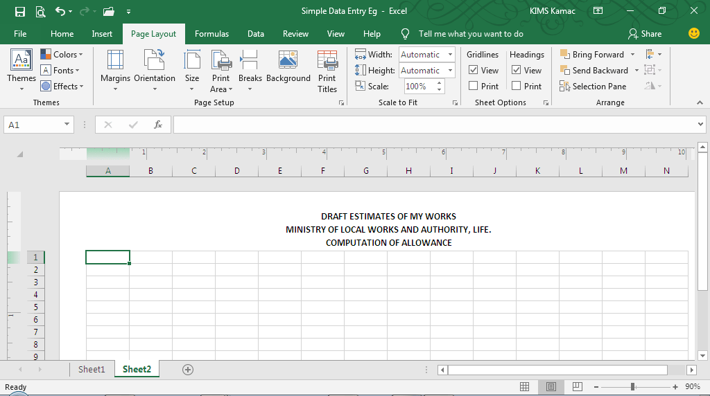

Now, we are ready to start entering data in the first and second rows.
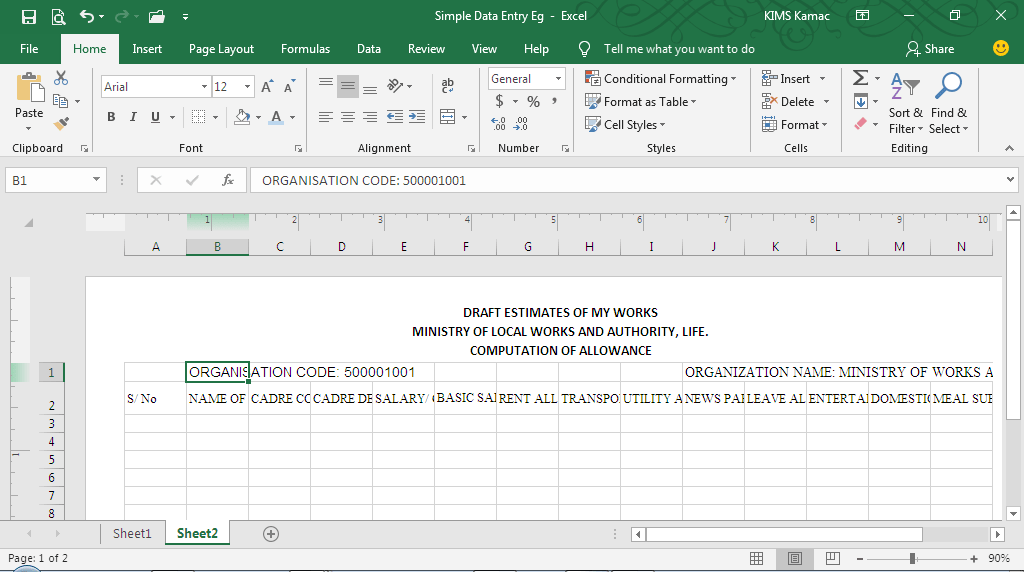
- Type ORGANIZATION CODE: 500001001 in cell B1, and ORGANIZATION NAME: MINISTRY OF WORKS AND LIFE in cell J2.
Note: The positioning of the above information must not be in the cells described. Just position them in any of the cells in the first row that will make the first to be in the left-hand side and the second in the right-hand side.
- Then type the following in row 2, beginning in cell A2 to P2: S/ No, NAME OF OFFICERS, CADRE CODE, CADRE DESCRIPTION, SALARY/ GROUP STEP CODE, BASIC SALARY (N), RENT ALLOWANCES, TRANSPORT ALLOWANCES, UTILITY ALLOWANCES, NEWSPAPER ALLOWANCES, LEAVE ALLOWANCES, ENTERTAINMENT ALLOWANCES, DOMESTIC STAFF ALLOWANCES, MEAL SUBSIDY/PA. ALLOW, MEDICAL ALLOWANCES, TOTAL. After typing in the data, your work should look like this:

- Next, bold the entries in row 1 and row 2. Then, in row two, apply the following formatting: centralize the data, reduce the font size to 8pts, adjust the column width of some columns, and wrap the texts to ensure that they are all seen. After the customizations, you will have:


- Start entering data on the rest of the cells. Merge cells where necessary and apply superscripts to texts where necessary.
- After entering the data on all the pages, apply a
border to the pages as follow:
- Highlight all rows that contain data, except the first row.
- In the Home tab, locate borders icon and select it. From the dropdown list, select all borders.
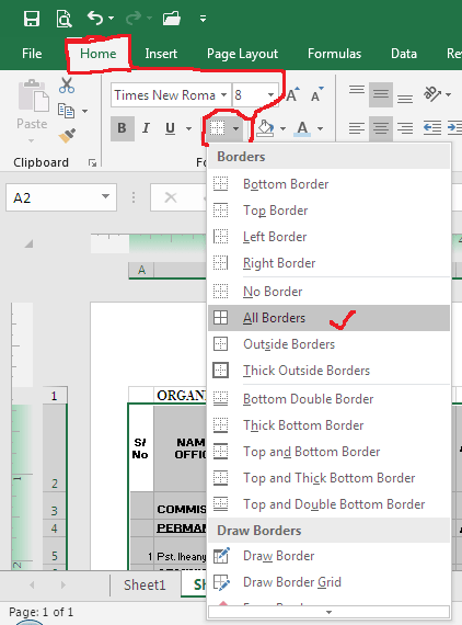

- After the border has been applied, the work will look like this:
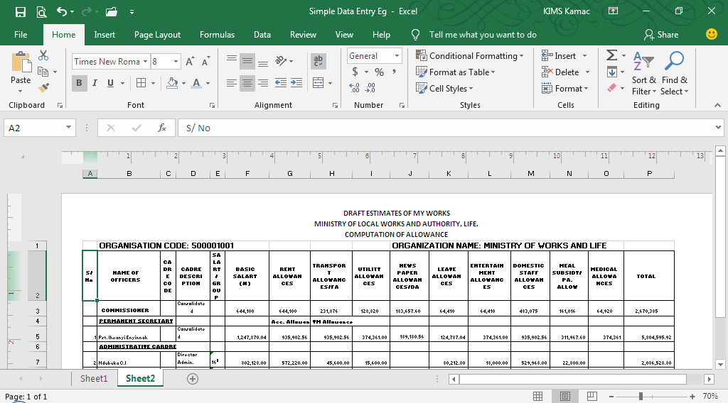

- Switch back to the normal view. You have successfully accomplished the task of entering data for presentation.
If there is any question, or if you encounter difficulty at any point, kindly ask a question in the comment box below.
Data Entry for Printing – Invoice template
In this third example, we will be creating an invoice template for printing. When a client or customer buys goods from a company, an invoice is usually issued to the customer/client. After this template is created, any business can input its name and the products’ sold, and then issue it to a customer/client.
Let us begin this way:
- Set up your page to the size you want: Letter, A4, Statement, Executive, … We will use the Letter paper size.
- Select the Page Break Preview and return back to the Normal view. This will demarcate the pages of the worksheet so that you can work on a page at a time. You will see dotted lines drawn across the worksheet as shown below:


- Select cell A1 and adjust the column width and row height as follow: make column width = 44 and row height = 88.
- Select cells B1, C1 and D1 and make their column width = 12.
Remember: to change column width or row height, in the Home tab, under Cells group, click Format, and select Column Width or Row Height. Then fill in the dialog box with the above-specified values.


- Select cell A1 and
insert a company’s logo in the cell. To do this, follow the following steps:
- Select cell A1. On the Insert tab, click Illustrations and select Pictures.
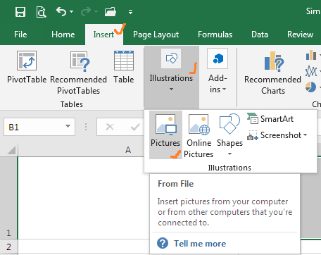

- From the Insert Pictures window, select a picture for your logo. Then resize the picture logo to fit inside the cell.
- Select the picture logo, in the Format tab, under Arrange, click the Align Objects icon, and select Snap to Grid.


- Select cells C1 and D1 and merge the cells together. In the merged cell, type: SALES INVOICE. Then align the text right center.
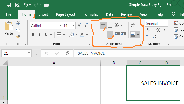

- In cells A2 – A6, type the following: COMPANY NAME, No of street address, Location (Town/City), State/country, and Tel. No.
- In cells C2 and D2 type: Invoice No. and 0000111. Then, merge cells C4 and D4, and C5 and D5. In merged cell C4/D4, type CUSTOMER NAME.
- In cells A8 – A15, type in the following, Customer Billing Address, Name of Contact Person, Company name, Street Address, Location (Town/ City), State/ Country and Tel. No., but jump A9 and reduce its row height.
- In cells C8 – C14, type in the following: Customer Shipping Address, Contact Person, Company name, Street Address, Location (Town/ City), and State/ Country, but jump A9.
- Your work should look like this by now:
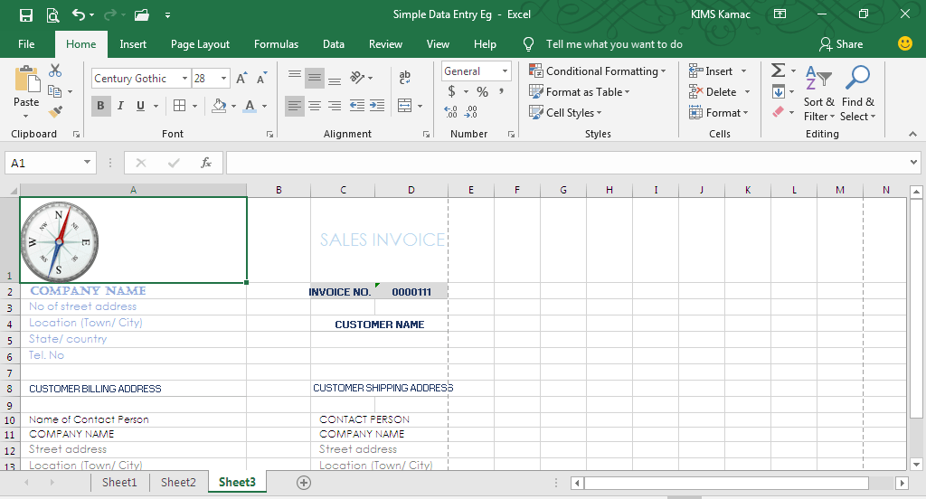

- Then complete the remaining cells following the diagram below:
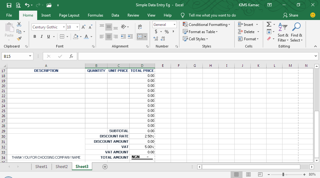

- If
you have completed the template following the information above, then let’s
finish the work by adding borders and formula:
- In cell D18, type the formula: =PRODUCT(B18, C18). Use the autofill handle to fill it through to D28.
- In cell D29, enter the formula: =SUM(D18:D28)
- In cell D30, enter 2.5%; in D31 enter: =D30*D29
- In D32, enter 5%; in D33 enter: =PRODUCT(D32,D29); and in D34, enter =D29-D31+D33.
- Before we apply a border, in the View tab, under Show, deselect Gridlines as shown below.


- Then, select cells C2 and
D2, and apply
fill color to
them.
- Select cell C5/D5 and apply top and bottom borders. Follow the same pattern to apply borders to all the cells that require border. You can customize it as per your choice.
We are done with the template; your work should look similar to this:


If you are confused at any point, ask your questions in the comment box below. If you want any special topic on Excel explained, which we have not already discussed, communicate us through the comment box or the contact page.

