Your cart is currently empty!
Category: InfoComTech
Information technology has changed business processes, information management, information dissemination, and commerce in recent times. Virtually everything we do has a link with technology.
Learn coding and programming the easy way. The knowledge you need to unmask your creativity and creative ability.
How to Make Pie Charts in Excel: Bar and Line Charts
To make pie charts in Excel is simple, just as to make other types of charts. Pie charts represent data categories in proportions, though it is not suitable for all kinds of data.
In Microsoft Excel and other spreadsheet applications, charts help us to summarize data. A well-created chart or graph helps data consumers to analyze trends, spikes, and data patterns at a glance.
Sometimes, data could be cumbersome and difficult to analyze, but with charts, you can easily visualize the trends and patterns. Available charts in Excel will allow you to represent data in a variety of ways. You can choose between column, line, pie, bar, and many more charts suitable for your data.
Making professional-looking charts in Excel and other spreadsheet applications is easy. All you need to do is to choose a chart type, a chart layout, and a chart style.
For example, to make pie charts in Excel, you start by entering the data for the chart on a worksheet. Then select the data and choose a pie chart from the Charts group on the Insert tab. The chart appears as shown in the figure below.
Excel supports numerous types of charts to help you display data in ways that are meaningful to you and your audience. In this tutorial, you will learn how to make charts in excel, including pie, bar, and line charts.
Types of Charts in Excel
Microsoft Excel 2016 has about 15 types of charts you can choose from. The type of chart you can choose to represent your data depends on the nature of your data. Let us list the different types of charts in Excel 2016 and the nature of the data suitable for them.
S/n Types of Charts in Excel 2016 Use Case 1 Column charts (vertical bars) Use to compare values across different categories 2 Bar charts (Horizontal bars) Use to compare values across different categories, especially, when categories name is long 3 Line charts Use to display trend values over time, especially, when there are many data points 4 Area charts Use to display trend values, especially, when there is a need to highlight the magnitude of change over time. 5 Pie charts Use to show the proportion of a category from the whole. The whole equals 100%, each proportion is derived from the 100%. 6 Treemap charts Use to compare values arranged hierarchically using different rectangular levels, especially, when there are few categories 7 Sunburst charts Use to compare values arranged hierarchically using a ring, especially when there are many categories of data 8 Histogram charts Use to display the distribution of data 9 Box and whisker Use to display the variations within data categories 10 Scatter charts Use to show the relationship between two sets of data 11 Waterfall charts Use for financial data to show the cumulative effect of a series of positive and negative values 12 Surface charts Use to show trend values across two dimensions 13 Radar charts Use to show values relative to a center point 14 Stock charts Use to display the trend of stocks or forex over time, especially when there are different price values 15 Combo charts Used to combine two charts for two different values to highlight different types of information How to make charts in Excel
Charts or graphs are graphical representations of data. Charts are used to summarize large tabular data for easy understanding. It also shows the relationship between the different parts of the data.
In Microsoft Excel, there is a Recommended Charts command; this command helps a user to choose the appropriate chart for the data in the view.
To create charts in Excel, do the following:
- Select the range of data you want to create chart on.
- Select the Insert tab.
- On the Insert tab, under Charts group, select Recommended Charts or choose any chart type of your choice.
- The selected chart is automatically plotted and displayed for you, based on the selected data.
How to make Pie Charts in Excel
Pie charts are circular graphs used to represent numerical proportions of data in slices. Pie charts represent proportions of categorized data in percentages.
To make pie charts in Excel, your data should be categorized. For example, the geographical distribution of sales, gender distribution of students, departmental distribution of salaries, etc.
To illustrate how to make pie charts in excel, let’s use the following table. The table shows the level of students’ responses in a Chemistry class of 87 students. Let us make pie charts using the data.
Response No. of Students Very Positive 15 Positive 18 Neutral 20 Negative 9 Very Negative 25 To make pie charts in Excel, do the following:
- Enter the above data in a worksheet. You can also copy and paste the data in a worksheet.
- Select the range of data, as shown below.
- On the Insert tab, under Charts group, select the Pie Chart icon.
- From the list, choose any of 2-D Pie, 3-D Pie or Doughnut. Your chart is displayed as shown below.
- Select the chart title, delete the current title and replace it with an appropriate chart title.
- You can also change the chart style from the Chart Design tab to a suitable style.
- Perform other editing tasks as explained under editing and formatting charts.
How to make Bar Charts in Excel
Bar charts in Excel use vertical or horizontal rectangular bars of different heights to represent categorized data. The lengths of the rectangular bars are proportional to the values they represent.
Microsoft Excel differentiates between column charts and bar charts. Column charts use vertical rectangular bars to represent data, while bar charts use horizontal rectangular bars. Both can be used for the same kind of data. Bar charts are usually recommended if the category titles are long.
To make bar charts in Excel, do the following:
- Enter the appropriate data in a worksheet.
- Select the range of data you want to use to plot a bar chart.
- On the Insert tab, under Charts group, select the bar Chart icon. NB: You can also select Recommended Charts to display the list of charts suitable for the selected data. Select either column or bar chart from the list.
- If you selected the bar charts icon, from the list, choose any of 2-D column, 3-D column or 2-D bar or 3-D bar. Your chart is displayed.
- Select the chart title, delete the current title and replace it with an appropriate chart title.
- You can also change the chart style from the Chart Design tab to a suitable style.
- Perform other editing tasks as explained under editing and formatting charts.
How to make line charts in Excel
Line charts in Excel are a series of data points that are connected together with a straight line. Line graphs are suitable for trend values. They represent data points over time, e.g., years, months, or days.
To make line charts in Excel, do the following:
- Enter the data in a worksheet.
- Select the range of data you want to use to create line charts.
- On the Insert tab, under Charts group, select the line Chart icon. NB: You can also select Recommended Charts to display the list of charts suitable for the selected data. Select a chart from the list and click OK.
- From the dropdown list of line charts icon, choose any of 2-D line, 3-D line or area chart. Your chart is displayed as shown below.
- You can change the chart style from the from the Chart Design tab to a suitable style.
- Perform other editing tasks as explained under editing and formatting charts.
Editing and formatting Charts
When you make charts in Excel, two more tabs are added to the list of tabs in MS Excel. These tabs are Chart Design and Format tabs. NB: The chart must be selected in order to display these two tabs.
- The commands on the Chart Design tab are used to edit the look of the created chart automatically.
- The commands on the Format tab are used to edit the individual texts, lines and shapes of the chart.
How to Edit charts in Excel
To edit charts in Excel, do the following:
- Select the chart to display the chart editing tools, see image below.
- Click the “plus-like” icon to display the Chart Elements list. The items on the list depends on the type of chart selected.
- Select any of the items on the list to display the element on the chart. e.g., select the Chart Title to display a title for your chart.
- To edit a displayed element, click to select it, then type a suitable text in the selected box.
- Click on the arrow at the right of the selected item to display the item’s properties. e.g., you can place the Legend at any of Top, Bottom, Left or Right positions.
- Click the “brush-like” icon to display the Style and Color properties of the chart.
- Under the Style tab, select a style of your choice to see your chart’s properties change.
- Under Color tab, select a color scheme of your choice to see the chart’s colour scheme change.
- Click the “funnel-like” icon to display the Values and Names properties of the chart.
- The Values tab is split into Series and Categories. To remove or add any item on the Series and Categories, deselect or select such item and click Apply on the down-left corner of the list.
- For example, to remove positive category on the pie chart above, deselect the positive option button and click Apply.
- Therefore, you can decide to show or not show the values of the categories or series on your chart.
- Finally, you can use the Names tab to display the titles used on your data table on the chart or not. E.g. If you do not want to display the names on the categories list, select (None) and click Apply.
Change the location of a chart in a workbook
- Click the chart to select it and to display the chart design tab.
- On the Chart Design tab, in the Location group, click Move Chart.
- From the dialog box that appears, under Choose where you want the chart to be placed, do one of the following:
- To display the chart in a chart sheet, click New sheet.
- To display the chart as an embedded chart in a worksheet, click Object in, and then click a worksheet in the Object in box.
Save charts in Excel as a chart template
- Right-click the chart that you want to save as a template.
- From the popup list that appears, select Save as Template.
- In the Save in dialog box, make sure that the Charts folder is selected.
- In the File name box, type an appropriate name for the chart template and save.
- To create a new chart based on the graphs template, do the following:
- Select the range of data.
- On the Insert tab, under Charts group, select Recommended Charts.
- On the Recommended Charts dialog window, select the All Charts tab.
- From the list of chart types, select Templates folder.
- Select the charts template you want to use to create your chart and click OK.
Conclusion
Charts are data analysis tools that help us to summarize, visualize and compare data with ease. Microsoft Excel provides different types of charts that are suitable for different categories of data.
To make charts in excel is easy and straight forward as explained in the sections above. Though we did not illustrate how to create all types of graphs in Excel, the steps are the same. No matter the type of chart you want to create, follow the steps on how to make charts in Excel.
We also added here how you can customize your charts using chart editing tools. The tools explained are handy when you use them through the ribbons command. The Chart Design tab makes it easy to edit charts in Excel. I believe that this tutorial has helped you to learn how to make bar, line, and pie charts in Excel. If you have questions, please, kindly forward them.
How to use PivotTable in Excel 2016
PivotTable in Excel is an advanced tool that allows you to organize and analyze large data set. Using pivot tables, you can extract data from a large dataset, and present the summary or analysis of such data.
PivotTables help you to easily see patterns and trends and easily make comparisons of data in a table. You can easily summarize large data using functions such as Sum, Count, Average, etc.
For example, the Pivot Table below summarized the number of students registered for the new section in a given secondary school. A total of 258 students were registered into different classes from SS1 to SS2.
Pivot Tables Explained
PivotTables are used to summarize data, especially, when the available data is large. With it, you can easily identify variations and seasonality in data. You can also view data from different perspectives with just a click using PivotTables.
For example, in the above table, we can view the total number of registered students by sex or by class.
PivotTable in Excel 1993 – 2007
Pivot table has been part of Microsoft Excel since 1993 when it was included in Microsoft Excel 5. Since then, Microsoft has improved on the functionality of the pivot table as new versions of Excel are released.
For instance, The Excel 1997 version included the pivot table wizard and the ability to create calculated fields. The Excel 2000 version added a pivot chart to graphically represent pivot table data.
In 2007, the Excel version improved how to work with PivotTables by making it a lot easier to work with. It becomes easier to interact with the fields on the pivot table workspace.
PivotTable in Excel 2010
In 2010, a new feature was added that assists users to quickly customize pivot tables with a click. Then, you can easily change pivot table summary types and calculation types from the ribbon with a click.
PivotTable in Excel 2013
In 2013, a timeline was added to pivot tables. Timelines allow you to filter records in a PivotTable by dates.
To add a timeline in Excel 2013, select the PivotTable and click on the contextual Analyze tab. Under the filter group, select insert timeline. A dialogue box appears from where you will customize your timeline.
PivotTable in Excel 2016
In 2016, the search field was included in the pivot table. This makes it easier to search for fields within the pivotable, especially, when working with many fields. It also eliminates confusion, saves time, and makes working with fields in the pivot table easier.
PivotTable in Excel has witnessed a lot of improvements since its inception. These improvements have made working with PivotTables easier and made the skill important among Excel users.
What is the use of PivotTable in Excel?
Generally, a pivot table is used to organize a large volume of data so anyone can easily understand them. The use of a pivot table depends on the volume of data and what the user wants to achieve.
Looking at the above example as a guide, we can say that the uses of PivotTables include the following:
- To summarize a large volume of data. For example, the registered students were summarized using Sex and Class. Generally, we can easily deduce the number of students that were registered, and the number in each class.
- To sort and filter data. The pivot table provides an option that assists users to sort data in ascending or descending order. You can also decide to filter data using data labels or based on categories.
- To organize and reorganize data into groups or categories. You can organize data in columns and rows, and reorganize data in rows and columns using different fields. To achieve this, you can simply add fields to column or row labels.
- To analyze data with the aid of functions. The summary of the data can be obtained by performing necessary calculations using preset functions. The values field allows you to select any function of your choice to summarize your data. You can use the SUM, COUNT, AVERAGE functions, etc. In our example above, we used the COUNT function to summarize our data.
- To perform data comparison. You can compare data by using a multi-dimensional table to figure out differences and trends in data units.
How to create a PivotTable in Excel 2016
To create a PivotTable in Excel, especially Excel 2016 and 2019, do the following:
- Open the worksheet that has the data you want to summarize or type the data in a worksheet. If you wish, convert the data to a table.
- Select a cell anywhere outside the data table. Though you can choose to insert the pivot table in another worksheet.
- On the Insert tab, under the Tables group, select PivotTable.
- The PivotTable dialog box appears.
- On the PivotTable dialog box, under Table/Range enter the name of the table or highlight the entire data range.
- On the dialog box, under Choose where you want the PivotTable to be placed, select Existing worksheet. Then select a cell location within the worksheet. See the image above.
- Click OK on the dialog box to display PivotTable fields and PivotTable workspace.
- On the PivotTable fields, select the fields you want to display. Move any of the fields to the rows or columns depending on how you want the summary.
- To filter the results, move a field to the filter area.
- To compute the summary of the data, move the summary field to the values area and choose a function. When you move a field to the values area, the COUNT or SUM function is automatically selected.
- The results of the selected fields are displayed in the PivotTable report workspace as shown below.
PivotTable Example
Haven understood how to create a PivotTable in Excel, let us illustrate how to use the PivotTable.
The worksheet below shows the sales record of Bluewy Inc. for September. Use the pivot table to analyze the data.
Firstly, let us create the PivotTable using the above steps. The image below displays the PivotTable Example using the Bluewy sales record.
On the PivotTable, we can perform the following as discussed above. Sort data, filter data, summarize data, and compare data.
Sort data in PivotTable
On the PivotTable report workspace, right-click a cell under Sum of Sales. And point to Sort. Select either ascending order or descending order.
You can also click the Row Labels and sort either ascending or descending order. You can also filter based on the rows categories.
Filter data in PivotTable
Add a field in the filter area of the pivot table field. We added a region in the filter area.
On the PivotTable report workspace, click the filter button and select any of East, South, or West and click OK.
Perform data comparison
To create a multi-dimensional table and make a data comparison you will add a field in the row area and another in the column area.
In the Pivot table above, move regions to the column area and Sales reps to the row area. You have created a multi-dimensional table that will help you compare the sales in different regions and sales reps.
Conclusion
The PivotTable is a skill that is important in today’s world. This has made it necessary for students, applicants, and users of Excel to seek its knowledge.
The tutorial thus far has illustrated how to use PivotTable in Excel. It is quite simple to create a pivot table for any use you want.
INDEX MATCH Function with Multiple Criteria In Excel
The INDEX MATCH function is used to perform a two-way lookup to extract values from a data table. It is used as a substitute to vlookup multiple criteria in Excel before the introduction of the xlookup function.
Remember that the vlookup function cannot perform vertical and horizontal lookup at the same time. To perform a multiple criteria lookup in Excel 2019 and lower versions, we employ the INDEX MATCH MATCH function.
INDEX MATCH function combines two Excel lookup and reference functions category – the INDEX function and the MATCH function. The INDEX function returns a value using a known row and column number. But the MATCH function returns the relative position of a specified item within a range.
When both functions are combined, we can return a value using vertical and horizontal arrays. This helps us to perform a lookup with multiple criteria in Excel without using the VLOOKUP or HLOOKUP functions. In this tutorial, you will learn how to use the INDEX MATCH MATCH formula.
INDEX Function in Excel
The INDEX function is used to return a value within a range in a worksheet. To use the INDEX function, data will be arranged in rows and columns. And each row and column will be numbered from 1 – n.
For example, the table below shows the list of students in a given class. The columns are numbered 1 to 5 and the rows are numbered 1 to 10.
1 2 3 4 5 Row/ Column Nos. S/N Student Name Sex Class First Term 1 1 Emma Akin Male SS2A 92 2 2 Udo Mark Female SS2B 58 3 3 Martin Greg Male SS2A 65 4 4 Amaka Prince Female SS2B 85 5 5 Peace Evere Male SS2C 57 6 6 Ebere Golden Male SS2A 69 7 7 Umaru Mary Male SS2B 68 8 8 Vilva Friday Female SS2A 86 9 9 Monday Tony Female SS2C 92 10 To use the index function to return a value in a range or table, you will specify the array and the row and column numbers.
Syntax of the INDEX function
The INDEX function is given by the following:
=INDEX(array,row_num,[column_num]) – array form =INDEX(reference,row_num,[column_num],[area_num]) – reference form
Where;
- array is required. This is a range of cells from where a value will be returned. If one row is selected, the row_num is optional, similarly, if one column is selected, the col_num is optional.
- reference is required. This is representing a reference to one or more ranges of cells from where a value will be returned. If the references to the ranges are non-adjacent, enclose them in parenthesis, e.g. (A2:B5, A10:B15). If each area in the reference has only one row or column, then the row_num or column_num is optional.
- row_num is required if a column is present. This is the row number in the array or reference from where a value should be returned. It is optional if only one row is selected.
- column_num is required if a row is present. This is the column number in the array or reference from where a value should be returned. It is optional if only one column is selected.
- area_num is optional. This is the area number of the reference from where a value should be returned. According to how the areas are selected, the first area becomes area_num 1, the second area, area_num 2, etc.
The second INDEX formula is called the reference form. It is usually used when area references are from non-adjacent selections. In this case, we enclose the areas with a parenthesis. Let us use the worksheet below to illustrate.
In the above worksheet, I can include only the following fields: S/N, Student name, Sex, and Exam score, and Remark. This will result in the following areas: A1:C20, and E1:F20. Where A1:C20 is area_num 1, and E1:F20 is area_num 2.
Therefore, to return the student’s exam score in row 7, the formula will be =INDEX(($A$1:$C$20,$E$1:$F$20),7,1,2). Where $A$1:$C$20 is area 1, and $E$1:$F$20 is area 2. The row_num is 7, and the value to return is located in column_num 1 of area_num 2.
Example of the INDEX function
The worksheet below shows the number of students in SS2 offering different courses. Using the index formula,
- How many students in SS2D are offering Mathematics?
- How many students are offering Economics?
Solution
To solve the above problem, let us do the following:
- Create a worksheet with the above data
- Number the columns and rows: there are 12 rows and 6 columns
- Select the cells where the results will appear (see solution below).
- For No. of students offering Mathematics in SS2D, enter the formula: =INDEX($A$1:$F$12,4,5). Note that: the row_num is 4 and the column_num is 5, using the given array.
- For the total number of students offering Economics, enter the function: =SUM(INDEX($A$1:$F$12,7,0,1)). Note that: we used the reference form where 7 is the row_num, 0 the column_num, and 1 the area_num. We used the sum function to get the total for row 7 which is Mathematics.
The result of the above solution is shown in the image below.
MATCH Function in Excel
The MATCH function is used to return the relative position of a specified item within a range of cells. In this case, the required item is known but the position of the item within a range is not known.
Like in the INDEX function, the MATCH function will automatically number the items in a selected range. It will then return the position number of the item you are searching for. For example, in the table below, the position of Biology is 5, and SS2B is 2, depending on the selected range.
1 2 3 4 5 SS2A SS2B SS2C SS2D SS2E 1 English Lang. 48 45 49 52 47 2 Lit. in English 21 24 26 35 40 3 Mathematics 48 45 49 52 47 4 Chemistry 32 34 21 15 16 5 Biology 34 40 43 48 45 6 Economics 47 20 34 41 43 7 Civic Education 41 32 32 25 34 8 Physics 43 28 36 43 35 9 Animal Hus. 35 41 35 34 26 10 Agric. Science 42 43 35 26 27 11 CRS 15 24 16 35 30 Therefore, when you know the item, you are looking for, but want to find its position, use the MATCH function.
Syntax of the MATCH function
The MATCH function is given by the following: =MATCH(lookup_value,lookup_array,[match_type])
Where;
- lookup_value is required. It represents the item or value you want to know its position in the lookup_array. For example, SS2B, in the table above. SS2B is the lookup_value. The lookup_value can be a text, number, or cell reference,
- lookup_array is required. This represents the range of cells from where to search for the lookup_value.
- match_type is optional. This option will tell Excel how to match the lookup_value. There are 3 options:
- 1 – This is the default match_type. It finds the largest value that is less than or equal to the lookup_value. When used, the items in the lookup_array MUST be arranged in ascending order. If match_type is omitted in the MATCH function, this option takes effect.
- 0 – This option is used to search for the exact match of the lookup_value. If there is more than one match, the position of the first value will be returned.
- –1 – This option finds the smallest value that is greater than or equal to the lookup_value. When used, the items in the lookup_array MUST be arranged in descending order.
Example of the MATCH function
The worksheet below shows the number of staff in ABC Logistics. Use the match formula to locate the position of the Marketing department.
Solution
To solve the above, let us do the following:
- In the worksheet, specify a cell where the result will appear. Let the lookup_value appear at the top or to the left of the output cell.
- On the output cell, enter the formula: =MATCH(J10,$J$1:$J$8,0). Note: Select the lookup_value on the left of the output cell (J10). Then select the lookup_array which is ($J$1:$J$8); finally, specify the exact match which is 0. Press ENTER to display the result.
- The value returned is 7. Remember that this is the relative position counting from the top, not the no. of staff in the dept.
INDEX MATCH Function in Excel
Looking at the INDEX and the MATCH functions, you will observe that they are opposite of each other.
This means that if we don’t know the row_num and the column_num, we can use the MATCH function to get them. This brings us to INDEX MATCH in Excel.
In INDEX MATCH in Excel, we use the MATCH function to provide the row_num or column_num within the INDEX function. To use the INDEX MATCH function in Excel, we rewrite our function as follow:
- =INDEX(array,MATCH(lookup_value,lookup_array,[match_type]),column_num). Here, the row number is unknown but the column number is known.
- =INDEX(array,row_num, MATCH(lookup_value,lookup_array,[match_type])). Here, the column number is not known but the row number is known
- =INDEX(array,MATCH(lookup_value,lookup_array,[match_type]), MATCH(lookup_value,lookup_array,[match_type])). Here, both row and column numbers are not known.
Let us illustrate how to use each of the above formulas with examples.
Index Match with Multiple Criteria:
The INDEX MATCH with multiple criteria is simply using the INDEX and MATCH function for a two-way lookup. To illustrate this, we use two examples where the row number is known and the column number unknown, and vice versa.
Example of Index Match multiple criteria rows and columns
The worksheet below displays the number of staff in a Classical Secondary School, Ipanja. The teachers’ names are arranged based on qualifications.
Use the INDEX MATCH function to solve the following:
- The number of teachers that studied Medical Science.
- The number of teachers that have MBA.
- Find the number of B.SC holders that teach Mathematics
- The number of teachers in the Education Department that have TC II qualifications.
Solution
The solution of the above questions will help us understand how to apply the INDEX MATCH and INDEX MATCH MATCH. Take the following steps.
1. In the worksheet, specify cells where the results will appear. (See the output below).
2. For question No. (1), enter the following formula in the output cell: =SUM(INDEX($B$2:$K$18,0,MATCH(B23,$B$1:$K$1,0)))
- In this example, the MATCH function is used to return the column_num in the INDEX function.
- The SUM function calculates the total No. of teachers.
- The INDEX function is used to select the area that will be calculated.
- The MATCH function nested in the INDEX function is used to select the column that will be calculated. The result is shown in the image below.
3. For question No. (2), enter the following formula: =SUM(INDEX($B$2:$K$18,MATCH(E23,$A$2:$A$18,0),0,1))
- In this example, the MATCH function is used to return the row_num in the INDEX function.
- The SUM function calculates the total No. of teachers.
- The INDEX function is used to select the area that will be calculated.
- The MATCH function nested in the INDEX function is used to select the row that will be calculated. The result is shown in the image below.
4. For question No. (3), enter the following formula: =INDEX($A$1:$K$18,MATCH(B28,$A$1:$A$18,0),MATCH(C27,$A$1:$K$1,0))
- In this example, the INDEX MATCH MATCH function is used to return the row_num and column_num.
- The INDEX function is used to return the number of B.Sc holders that teach mathematics.
- The result is shown in the image below.
5. For question No. (4), enter the following formula: =INDEX($A$1:$K$18,MATCH(B28,$A$1:$A$18,0),MATCH(C27,$A$1:$K$1,0))
- In this example, the INDEX MATCH MATCH function is used to return the row_num and column_num.
- The INDEX function is used to return the number of TC II holders that teach Education in the school.
- The result is shown in the image below.
Index Match Vs Vlookup
The vlookup function cannot be used to perform a lookup for multiple criteria. To overcome this limitation, we can use the INDEX MATCH functions. This is especially useful for those who are using Excel 2019 and lover versions. If you are using Excel 2021 or Microsoft 365, you can leverage the Xlookup function.
Hence, with the Index Match, you can do more than use the vlookup function. Meanwhile, the vlookup is still relevant for a one-way lookup to avoid unnecessary complications. It is, therefore, necessary to understand when to use any of the functions.
Conclusion
The Index Match function is a way of performing a multiple criteria lookup that does not exist in Vlookup. Therefore, it is important to understand when to use the vlookup and Index Match function to return a value.
There are various use cases where you can deploy the Index Match formula in Excel. All you need is to understand how to use it as explained above.
I believe that this tutorial has helped you build a foundation on Index Match vs vlookup functions. Continuous practice will help you improve and become an expert.
We are open to your questions in case you face any challenges working with the functions. We shall look at the pivot table in Excel by next week. Before you go, please, kindly share with a friend. Don’t forget to visit our previous tutorials if you have not done so.
What is Xlookup Function: Easy Vlookup Multiple Criteria
What is the difference between Vlookup and Xlookup functions? Vlookup and Xlookup functions are used to extract values in a table of data in Excel. Both are used to query a data table and extract items or values in an Excel table or range. The Xlookup function can be seen as a vlookup multiple criteria.
However, vlookup searches for its values from left to right while xlookup searches in a specified column. Also, vlookup cannot be used to extract more than one value, but xlookup can retrieve an array of values.
Just like the vlookup, the xlookup function is one of the functions in the Lookup and Reference functions category. It is used to search, locate and return an item/ value in a table or range of cells. The xlookup function allows you to look for a search term in a specified column. It will then return a result in a corresponding row from another column specified by the user.
For example, if we have the Reg. number of a student, we can search for and retrieve the student’s name. The difference between vlookup and xlookup here is that the lookup_value must not be in the first column. Therefore, the xlookup function searches for what you want in a range or array and returns the required value.
Let us illustrate with this simple example. The worksheet below displays the detail of students in SS1 in a given school. A random sample of 5 students was selected using their Class ID SS1A01, SS1A05, SS1B02, SS1C02, and SS1B07. Use the Xlookup in Excel to return the names of the students.
The xlookup formula in excel is written as follow: =XLOOKUP(Class_ID, the range to look for the value, the range where values will be returned from)
The above explanation will result in the following: =XLOOKUP(H2,$D$2:$D$23,$B$2:$B$23).
Note the following:
- The H2 is the cell reference of the first Class ID. If you copy the formula to the remaining cells, all the results will appear accordingly. You may decide to use each class id instead of cell reference if you are dealing with a few values. In this case, you will have =XLOOKUP(SS1A01,$D$2:$D$23,$B$2:$B$23).
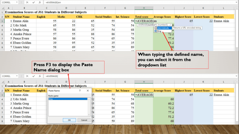
- The absolute range reference, $D$2:$D$23, references the range that contains the value we are searching for. We used absolute reference style so that when we copy the formula, the range will not change. You can also name the range. If you name the range, you will have something like this: =XLOOKUP(F3,Search_range,Return_range).
Where the Search_range is the name of the range to search, and Return_range name of the range to return a value. Naming the range allows you to copy the formula without changing the scope of the data.
- The last 3 entries not included in the function are optional. You can decide to omit them as we did and have the same result. We will talk about them later in the section for the syntax of the xlookup function.
The result of the vlookup formula is given below, check if your result is close to it.
What is Xlookup Function in Excel?
The xlookup function in Excel is one of the recently introduced functions in Microsoft Excel. It is available in Microsoft 365, Microsoft 365 for Mac, Excel for the web, and Excel 2021. It is used to query data to retrieve a value based on available data input.
To use the xlookup formula, we can organize our data in columns and rows. There is no need to put the lookup value towards the left of the return value. The lookup_value column and return value column can assume any position in the data range.
Our example above shows that the lookup value can take any position. As a result, columns are not numbered from the left to the right, as we do in vlookup. Using the xlookup function, we can perform both horizontal and vertical matches as shown in the table below.
SS1A SS1B SS1C English 76.5 82.1 79.6 Mathematics 78.3 65.8 71.2 Chemistry 63.9 72.3 81.2 Biology 78.2 80.3 76.9 Economics 60.8 64.7 62.1 Physics 87.2 76.2 84.5 The table above shows the average examination score of students in SS1 for six subjects. We can use xlookup to retrieve the average score of each class for each subject. To retrieve a value in the above table using the xlookup function, we will use the nested xlookup function.
For example, in the above table, to retrieve the average Biology score, for SS1B, we use the formula: =XLOOKUP(F3,$A$2:$A$7,XLOOKUP(G2,$B$1:$D$1,$B$2:$D$7)). The result will be as follow:
Therefore, we can use the xlookup to perform the functions of vlookup and Hlookup at the same time.
The syntax of the xlookup in excel
The syntax of the xlookup in excel is given by: =XLOOKUP (lookup_value, lookup_array, return_array, [if_not_found], [match_mode], [search_mode])
Where:
- lookup_value is required. It must be specified and represents the value you are searching for, e.g. Class ID. This value can appear in any column in the table. The lookup value can be a number, a text, or a cell reference.
- lookup_array is required also. This represents the range or array to search for the lookup_value. The lookup_array can be a range of cells using absolute cell reference, a named table, or a named range.
- return_array is also required. This is the range or array that contains the value to be retrieved by the xlookup function. As in above, it can be a reference, named table, or range.
- if_not_found is optional. This is used to create a return value if the actual match for the lookup_value is not found. Instead of returning a #N/A error value when lookup_value is not found, use this option. You can specify a return value or a return text in this optional argument. For example, “Class ID not found”. Note: If this option is not specified, xlookup returns #N/A if lookup_value is not found.
- match_mode is optional. By default, xlookup searches for the exact match of the lookup_value. You will use this optional argument to specify the match mode if you do not want the default. There are 4 match modes in xlookup, namely: 0, -1, 1, and 2.
- 0 – This match mode returns the exact match of the lookup_value. If the exact match is not found, it returns #N/A or the value in the if_not_found option.
- -1 – This match mode returns the exact match. If an exact match is not found, it returns the next smaller item.
- 1 – This match mode returns the exact match. If an exact match is not found, it returns the next larger item.
- 2 – This match mode is used to return a wildcard match. ? is used for a single match and * is used for sequence match.
- search_mode is optional. Use this option to indicate how xlookup will search for the required items. There are 4 search modes: 1, -1, 2, and -2.
- 1 – This is the default search mode. It performs a search from the first item on the list.
- -1 – This search mode performs a search in the reverse order. It searches from the last item on the list.
- 2 – This search mode performs a binary search in ascending order. The list must be sorted in ascending order, else, it will return invalid results.
- -2 – This search mode performs a binary search in descending order. The list must be sorted in descending order, else, it will return invalid results.
Vlookup vs Xlookup in Excel
What are the differences and similarities between the Vlookup and Xlookup functions in Excel? The similarities include:
- Both are functions in the Lookup and References category
- Both are used to retrieve values in a range or table of data.
- Both are used to search for items in vertically tabulated data.
- Both search for an item in a specified range and return a value from a specified range.
- Both have the lookup_value as their first argument in their syntax.
Some of the differences between vlookup and xlookup are tabulated below.
VLOOKUP XLOOKUP Lookup_value must be in the first column of the table_array Lookup_value can appear anywhere in the table of data The return value must appear to the right of the lookup column The return value can appear anywhere in the table of data Searches for items vertically only Searches for items both vertically and horizontally Cannot be nested in another vlookup function Can be nested in another xlookup function Uses column index to indicate the column containing the return value Does not use column index, but return_array to specify column containing the return value Returns #N/A error if the value is not found Has a parameter to substitute for the #N/A error if the match is not found Returns one item at a time Returns an array of multiple items How to use Xlookup Function in Excel
The xlookup function is an easier function to use than the vlookup function. Because of its simplicity, every excel user should master its usage and use it in place of vlookup and hlookup functions.
We shall illustrate how to use the xlookup in Excel using the following examples. Remember, you should have Excel 2021, Microsoft 365, or Excel for the web to practice these examples.
Example 1: Retrieve multiple items
The worksheet represents the sales record of Ugobest Enterprises. Five products were selected from the sales record: Festo biscuit, Minimie 100g, Nibit, Coca cola, and Viva 190g. The management wants to know who sold them and the selling price. Use the xlookup function to retrieve the required values.
Solution
Unlike the vlookup function that retrieves one item at a time, xlookup retrieves an array of multiple items. To solve this problem, we follow these steps.
- Enter the required data in a worksheet or import the data from any source. Note: use Excel for the web if you do not have Excel 2021.
- Create three columns within the worksheet and label them accordingly. See the example above.
- On cell G3, enter the following formula =XLOOKUP(F3,$A$3:$A$52,$C$3:$D$52, “Don’t Exist”). Note: we are using the default match and search mode.
- Copy the formula to the other cells below G3 using the autofill handle.
Notice that both Sales Rep. and Selling price column are populated at once. The result is shown in the table below.
Notice that the function in the sales rep. the column is reflected in the selling price column. You don’t need to replicate them yourself. Note that the wider the scope of your return_array, the more the items to be retrieved.
Example 2: Using match mode
The table below shows the results of students in a given secondary school. The grade obtained by each student is distributed using the following table.
S/N Score Range Grade 1 85 – 100 Excellent 2 70 – 85 V. Good 3 60 – 70 Good 4 50 – 60 Pass 5 0 – 50 Fail The average score of each student is shown in the worksheet below. Use the xlookup function to grade each student based on their scores.
Solution
To solve this problem, we’ll first create a table for the lookup value using the range and the grades.
- Create the table for the lookup values and ensure that it is sorted in ascending or descending order as shown above.
- Under grades, in column I2, enter the following formula: =XLOOKUP(H2,$L$3:$L$7,$M$3:$M$7,”Undefined”,-1,1). This formula is valid for the first table arranged in ascending order (A-Z). The xlookup function will search for and return values equal to or less than the lookup_value from the return_array.
- If you are using the second table arranged in descending order (Z-A), then enter the following formula: =XLOOKUP(H2,$L$12:$L$16,$M$12:$M$16,1,1). The xlookup function will search for and return values equal to or more than the lookup_value from the return_array.
- Copy the formula to other cells using the autofill handle. The results are shown in the figure below.
Example 3: Combining xlookup with other functions
The worksheet below shows the monthly sales record of Uchekondu Group Llc for January and February. Use xlookup to:
- Get the product with the highest selling price, the region, and the sales rep. in January
- The product with the lowest selling price, the region, and the sales rep. in February
- The price of Kellog Corn flakes, Huggies 3, and Festo biscuit in the West in February.
Solution
The Solution to the above problems is straightforward. Only that we will include another function in the xlookup function. Firstly, create columns where the results of the search will appear, as shown in the worksheet above.
- On cell L3 under product, enter the following formula: =XLOOKUP(MAX($D$4:$D$53),$D$4:$D$53,$A$4:$D$53,”Wrong”,1,1). We used the MAX function to locate the maximum (highest) selling price. So our lookup_value is the maximum value. We then return the product, region, sales rep, and price associated with the highest selling price.
- Copy the formula above and paste it in cell L4, and change the MAX function to MIN. the formula is: =XLOOKUP(MIN($D$4:$D$53),$D$4:$D$53,$A$4:$D$53,”Wrong”,1,1). The MIN function locates the lowest selling price. Then the rest of the function returns items associated with the lowest selling price.
- In the third question, use the nested xlookup to get the intersection of the products and the West region. Enter the following formula in cell L8: =XLOOKUP(K8,$F$4:$F$59,XLOOKUP(“West”,$G$3:$I$3,$G$4:$I$59, “Error”)). Use the autofill handle to copy the formula downwards.
The result of the above solutions is given in the worksheet below. To download the workbook for the above examples, click here.
Conclusion
The xlookup function is easier to use than the vlookup function. It is also more useful since it can return an array of multiple items.
The xlookup function has a parameter that can be used to return a specified option if an error occurs. There are various use cases where you can deploy the xlookup formula in Excel. All you need is to understand how to use it.
I believe that this tutorial has helped you build foundational knowledge on how to use the xlookup formula in Excel. If you keep practicing, you will understand it more. We are open to your questions in case you face any challenges while your newfound function. We shall look at the INDEX MATCH functions by next week. Before you go, please, kindly share with a friend. Don’t forget to visit our previous tutorials if you have not done so.
How to use Vlookup Formula in Excel
The Vlookup formula in Excel can be used to extract values in a table of data. It is a useful function that is used to query a data table and extract items or values in an Excel table or range.
Vlookup means vertical lookup, and it’s one of the few functions in the Lookup and Reference functions category. The vlookup formula in Excel is used to search for and return a corresponding value in a different column within the same row.
For example, if we have the Reg. number of a student, we can search for and retrieve the student’s name. Therefore, the vlookup formula in Excel searches for what you want in a table or range and returns the required value.
Let us illustrate with a simple example. The worksheet below displays the detail of students in SS2 in a given school. A random sample of 3 students was selected based on their Reg. Nos.: 5, 11, and 16. Use the Vlookup formula in Microsoft Excel to retrieve the names of the students.
The vlookup formula in excel is written as follow: =VLOOKUP(Reg. No., in worksheet range, column no. in the worksheet range, [exact/Approximate match])
The above explanation will result in the following: =VLOOKUP(F3,$A$2:$D$21,2,TRUE).
Notice that:
- The F3 is the cell reference of the first Reg. No. (5). If you copy the formula to the remaining cells, all the results will appear accordingly. You may decide to use the Reg, No., instead of cell reference if you are dealing with a few values. In this case, you will have =VLOOKUP(5,$A$2:$D$21,2,TRUE).
- The absolute range reference $A$2:$D$21 references the range that contains the data we are searching for. We used absolute reference style so that when we copy the formula, the range will not change. You can also convert the range to a table or name the range. If you do either, you will have something like this: =VLOOKUP(F3,Random_search,2,TRUE), where the Random_search is the name of the range. If you used a table, then, =VLOOKUP(F3,Table1,2,TRUE). Naming the range allows you to copy the formula without changing the scope of the data.
- The value “2” is the column index or column number within the range where what I am looking for can be found. Looking at the worksheet, you find out that the student’s name is in column 2, counting from the left.
- The last entry is optional. You can decide to omit it and still have the same result. TRUE stands for approximate match and is the default value. FALSE means exact match. TRUE usually selects a value close to or less than what you are searching for. But FALSE selects the exact match of what you are looking for.
The result of the vlookup formula is given below, check if your result is close to it.
What is Vlookup Formula in Excel?
The vlookup formula in Excel is one of the legacy functions that has been part of Excel since its inception. It is one of the most used functions in the history of Microsoft Excel. It is used to query data to retrieve a value based on available data input.
To use the vlookup formula, we must organize data in columns. The data is usually arranged such that the lookup value is to the left of the return value. Columns are numbered from the left to the right, indicating the column indexes, as shown below.
Reg. No Student Name Sex Class 1 Emma Akin Male SS2A 2 Udo Mark Female SS2B 3 Martin Greg Male SS2A 4 Amaka Prince Female SS2B 5 Peace Evere Male SS2C 6 Ebere Golden Male SS2A To retrieve a value using the vlookup function, we will provide the column index. The column index represents the column number within the data range. For example, in the above table, to retrieve sex, the column index is 3.
When using the vlookup function in Excel, the retrieved value must be to the right of the lookup value. This means that if you are looking up student names to retrieve the Reg. No. Then, the Reg. No. must appear to the right of the student’s name.
The syntax of the vlookup function in excel
The syntax of the vlookup function in excel is given by: =VLOOKUP (lookup_value, table_array, col_index_num, [range_lookup])
Where:
- lookup_value is required. It must be specified and represents the value you are looking up for, e.g. Reg. No. The secret of using the vlookup function is that the lookup value MUST be in the column index 1. That is, it must be in the first column of the range of data specified in the table_array. In our example above, notice that the Reg. No appeared in the first column (Column A) of the range $A$2:$D$21. The lookup value can be a value, a text, or a cell reference.
- table_array is required also. This represents the range or table where the vlookup function will search for the lookup_value to retrieve the value. Remember that the first column in this range must contain the lookup_value. The table_array can be a range of cells using cell reference, a named table, or a named range. The value to retrieve must be inclusive in the table_array for the vlookup function to return a value.
- col_index_num is also required. This is the column number that contains the value to be retrieved by the vlookup function. Remember that the columns should be numbered from left to the right beginning with the column that contains the lookup_value. That is, within the table_array count from the left-most (that contains the lookup_value) to the column that contains the return value.
- range_lookup is optional. This is used to tell the vlookup function to look for an approximate or exact match of the lookup_value. It is a logical value of TRUE or FALSE which can be written as 1 or 0 respectively. TRUE is the default value and searches for the closest value specified in the lookup_value column. FALSE or 0 searches for the exact value specified in the lookup_value column.
The exact and approximate match in the vlookup function
Range_lookup = TRUE
To use the approximate match (TRUE) option in the vlookup formula, always sort the first column in ascending order. If the value is not sorted, the return value might be wrong. This is because vlookup will look for the value equal to or smaller than the lookup_value specified.
If the lookup_value is smaller than the least value in the first column (lookup_value column), then the function will return #N/A.
Let us illustrate with the following example. In the worksheet below, the score of the student will determine if he/she is promoted, demoted, or not promoted. The status table is given as follow:
Score Range Remark 0 – 50 Demoted 50 – 75 Not Promoted 75 – 100 Promoted In the worksheet below, I purposely started with 50 instead of 0 to illustrate how TRUE works. The vlookup formula is given as follows: =VLOOKUP([@Score],$G$8:$H$10,2,TRUE), with the following result.
Notice that all values below 50 have the status of #N/A. This is because the lookup_value is smaller than the value looked up in the table_array. It, therefore, looks for an approximate match and returns a #N/A error if it did not see any.
Also, notice that all scores below 75 have a status of demoted. This is because TRUE in the range_lookup will return values equal to or smaller than the lookup_value.
Range_lookup = FALSE
If the exact match (FALSE) option in the vlookup formula is used, vlookup will return the exact match. If the exact lookup_value is not found in the first column (lookup_value column), then the function will return #N/A.
For example, using the above example, change the TRUE in the range_lookup to FALSE, to get the following result:
Notice that only a score of 75 returned a correct status. Others displayed #N/A. This is because there is no exact match.
Important notice
When using the vlookup formula in Excel, it is necessary to do the following:
- Always sort the first column in the table_array (column that contains the lookup_value), especially when using approximate match. Remember that approximate match is activated when the range_lookup is TRUE or 1.
- Always use absolute referencing, or a named range, or a named table when defining the table_array. This is important, especially when you want to copy the formula to other cells.
- Always store values appropriately to avoid incorrect results. Store numbers as NUMBERS, date as DATE, and text as TEXT. If you store the number as text, you will get incorrect results.
- Use wildcard characters in the vlookup function when range_lookup is FALSE and lookup_value is a text. Remember that “?” matches a single character and “*” matches a sequence of characters. This can be used, when using the exact match (FALSE) in the range_lookup and the lookup_value is a text, if necessary.
How to use Vlookup Function in Excel
As one of the most used functions in Microsoft Excel, every Excel user must understand it. We shall illustrate how to use the vlookup formula in Excel using the following examples.
Example 1: Simple use case
The worksheet represents the sales record of a given trading company. Five products were selected from the sales record: Festo biscuit, Minimie 100g, Nibit, Coca cola, and Viva 190g. The management wants to know who sold them and the selling price. Use the vlookup function in Excel to retrieve the required values.
To solve this problem, we follow these steps.
- Enter the required data in a worksheet or import the data from any source.
- Create three columns within the worksheet and label them accordingly. See the example above.
- Select the entire range of cells that contain the data and name it salesdata. Ensure that the first column contains the products because this contains our lookup_value. This range is our table_array. Please, don’t include the headers, i.e. products, Region, etc in the table_array.
- Label the columns from left to right: we have 4 columns starting with Products as 1 and sales as 4. These are our col_index_num.
- On cell G2, enter the following formula =VLOOKUP(F2,salesdata,3,FALSE). Note: we are using an exact match.
- Copy the formula to the other cells below G2 using the autofill handle.
- On cell H2, enter the following formula =VLOOKUP(F2,salesdata,4,0). Note that you can use either FALSE or 0 for an exact match.
- Copy the formula to the other cells below H2 using the autofill handle.
The result is shown in the table below. Your result should look like this.
We were able to use the vlookup function to query our data table and retrieve the values shown above. This is a simple scenario.
Example 2: Using vlookup in the place of IF function.
The table below shows the results of students in a given secondary school. The grade obtained by each student is distributed using the following table.
S/N Score Range Grade 1 85 – 100 Excellent 2 70 – 85 V. Good 3 60 – 70 Good 4 50 – 60 Pass 5 0 – 50 Fail The average score of each student is shown in the worksheet below. Use the vlookup function in Excel to grade each student based on their scores.
To solve this problem, we create a table for the lookup value using the range and the grades as follow:
- Create the table for the lookup values and ensure that they are in ascending order as shown above.
- Create a column within the table above which contains the lower bound of each range. This column will be the lookup_value column and the first column in the table_array. Ensure that this column is arranged in ascending order, see worksheet above.
- Highlight the lower bound column and the grades column and convert them to a table. To do this, On the Home tab, under Styles, select Format as Table. From the designs that appear select any table design.
- Name the table in 3 above gradeTbl. To do this, select a cell in the table you created. On the Table Design tab, under Properties, change the table name.
- Under grades, in column I2, enter the following formula: =VLOOKUP(H2,gradesTbl,2,TRUE). The vlookup function will search for and return values equal to or less than the lookup_value from the table_array.
- Copy the formula to other cells using the autofill handle. The results are shown in the figure below.
Conclusion
The vlookup function in Excel is very useful, though it has its weaknesses. You can use it to do different things such as retrieve a value from a data table and merge two tables.
The vlookup function can also be used with an IF function to return a different value if an error occurs. There are various use cases where you can deploy the vlookup formula in Excel. All you need is to understand how to use it.
This tutorial has helped you to build a foundational understanding of how to use the vlookup formula in Excel. If you keep practicing it in different scenarios, you will understand it more. We are open to your questions in case you face any challenges while practicing how to use the vlookup function.
There are yet other lookup functions in Excel: The Hlookup and the recently added Xlookup. The Hlookup is like the vlookup function but looks up a value in the rows rather than columns. We shall look at the Xlookup function by next week. Before you go, please, kindly share with a friend. Don’t forget to visit our previous tutorials if you have not done so.
The IF Statement in Excel: Nested and IFS Function
The IF statement in Excel is one of the logical functions in Microsoft Excel. It is used to return values when used alone and when used alongside other logical functions. The IFS function in Excel makes it easier to use multiple conditions than the nested IF statements. It returns the value_if_TRUE for up to 127 conditions.
The IF logical function has three (3) arguments. It returns one of two values based on the stated conditions. The first, if the condition is TRUE and the second, if the condition is FALSE.
For example, if a set of data represents the scores of students in an examination. And the examination board discloses that students who scored 60% and above passed while those who scored below failed. Then, a student will either pass or fail depending on his/her score. Those who scored 60% – 100% passed while those who scored 0 – 59.99% failed.
In this tutorial, we shall discuss how to use the IF statement in excel, including nested IF statements and the IFS function.
What is IF Statement in Excel?
The IF statement in Excel is a logical function used to make a comparison to return a value. The IF function is used to compare a statement to know whether it is TRUE or FALSE. When creating an IF statement, the IF function usually has two values. The first value is returned when the compared value is TRUE, and the second is returned when the compared value is FALSE.
Take a look at the student exam scores shown in the worksheet below and the results of the IF statement.
Using the IF statement in Excel, you can easily determine those who passed and those who failed. You will achieve this by specifying the value when TRUE and the value when FALSE. For example, IF(value >=60, “Passed”, value <60, “Failed”).
Looking at the statement, you will understand that a student will either score >=60 or not. Hence, the condition will be either TRUE or FALSE. Therefore, the above statement can be rewritten as follow: IF(value>=60,“Passed”,“Failed”), indicating that a student will pass or fail based on his/her score.
The Remark column in the worksheet above is where we used the IF statement to display who passed or failed.
Syntax of IF Statement in Excel
The syntax for the IF statement in Excel is given by: IF(logical_test, [value_if_true], [value_if_false])
Where:
- logical_test: is a required condition that must be specified. This argument represents the condition that must be tested and evaluated to TRUE or FALSE. Such conditions can contain text, numbers, cell references, dates, logical operators, and functions.
- value_if_true: This is an optional argument. It represents a text, number, cell reference, date, or function that must be returned/evaluated when the logical_test is TRUE.
- value_if_false: This is an optional argument. It represents a text, number, cell reference, date, or function that must be returned/evaluated when the logical_test is FALSE.
In its simplest form, the IF statement gives you a value of YES/No depending on the result of the logical_test.
Uses of IF statement in Excel
As stated in our previous tutorial, logical operators output TRUE or FALSE values. But we can use them with the IF statement to output actual values. Hence, we use the IF statement in Excel to:
- Test if a condition is true or false, and output a value based on such test.
- To create conditional functions that must be evaluated based on stated conditions. IF statement accepts a function, therefore, we can evaluate a function based on a stated condition.
- To execute a task that will be triggered based on a value. We can use the IF statement to create conditional formatting which is triggered based on a specified value.
Generally, the IF statement can be used in any scenario that requires testing a condition that will evaluate to TRUE or FALSE.
Simple example
The simplest example of the IF statement is when used to evaluate a condition that results in YES or NO. The above example of Pass/ Fail is typical. Let us illustrate with the following examples.
- The worksheet above represents the sales of a named company. Sales 10000 and above attract commission while sales below 10000 do not attract commission. Use the IF statement in Excel to identify sales that will receive a commission.
- Sales made in the East have a higher sales margin while sales in other regions have lower margins. Identify all sales that attract higher and lower margins.
The solution to simple IF statements example
- Let us identify the sales with and without commission. We will mark sales with a commission “Pay com” and sales without commission as “No com”.
- In the worksheet, create another column called commission in cell F2.
- In cell F3, enter the formula: =IF(E3>=10000,”Pay com”, “No com”)
- Use the autofill handle to drag the formula to all the cells in the column.
- The cells with 10000 and above are labeled “Pay com” and others “No com” as shown below.
- Let us identify regions that have higher and lower margins. We shall mark regions with higher margins as “H-M” and regions with lower margins as “L-M”.
- In the worksheet, create another column called Sales Margin in cell G2.
- In cell G3, enter the formula: =IF(C3=”east”,”H-M”,”L-M”)
- Use the autofill handle to drag the formula to all the cells in the column.
- The cells corresponding to the East region are labeled “H-M” and others “L-M” as shown below.
These examples show a very simple way to use the IF statement in Excel. There are more complex scenarios, which we shall illustrate with examples below.
IF Statement Practice Exercises in Excel
How to use Nested IF statements in Excel
The nested IF statement is a system of using an IF statement in another If statement. When you have multiple conditions to test, you can use the nested IF statement to arrive at an answer. When the nested IF statement is used, you will specify the condition and value if true. The value if false is usually replaced with another IF statement until all conditions are entered.
For example, in the worksheet below, students are graded A – F based on their score in an exam as follow:
Score Range Grade 0 – 39.99 F 40 – 49.99 E 50 – 59.99 D 60 – 69.99 C 70 – 79.99 B 80 – 100 A Let’s use the IF statement to grade the students based on their exam score using the steps below:
- Create a column called Grades in column G.
- In cell G2, enter the following nested IF statement: =IF(E2<40,”F”,IF(E2<50,”E”,IF(E2<60,”D”,IF(E2<70,”C”,IF(E2<80,”B”,IF(E2<=100,”A”,))))))
- Ensure that the number of bracket closures equals the number of IF arguments used.
- Autofill the formula in the remaining cells in the column.
- Note the sequence of the arguments. The function executes from the first argument. If the first argument is TRUE, it stops, if it is FALSE, it moves to the next IF statement, and so on.
- The result of the nested if statements are given below.
The logic behind the nested IF statements is that if the first condition is TRUE, the true value is evaluated. But if the condition is FALSE, it evaluates another If statement until the end of the argument.
Using OR in IF statement in Excel
You can combine the IF statement with the OR logical function to output a value. This will enable you to test more than one condition at the same time. You can even combine the OR, and the AND functions together depending on the conditions being tested.
Example 2: OR in IF statement
Let us illustrate the OR in IF statement in Excel with the following example. Assuming that the management of Bluewy Inc. wants to give a 7.5% commission to sales made in the East region or sales above 10000. Then, the solution can be achieved as follow.
- Create a column called Paid commission. A commission of 7.5% of sales will be paid to East regions or sales above 10000, and none to others.
- In cell H3, enter the following formula: =IF(OR(C3=”east”,E3>10000),7.5%*E3,0)
- The formula states, if sales are made in the east region or sales are above 10000, pay a commission of 7.5% of the sales.
- Copy the formula to other sales in the column using the autofill handle.
- The result of the OR in IF function is given in the worksheet below.
Notice the amount of commission paid out, and the sales that received the commission.
Multiple IF AND Statement in Excel
Like the OR logical function, you can also use the AND logical function with the IF statement in Excel. With the AND function, you can verify or compare multiple values at the same time.
Example 3: IF AND statement
Let us illustrate the IF AND statement in Excel with the following example. The management of Bluewy Inc. wants to give a 9% commission to sales above 10000 made in the East region. This means that sales made in other regions do not count, and sales not greater than 10000 in the east region do not count. Do the following:
- Create a column called 9% commission. A commission of 9% of sales will be paid to sales above 10000 made in the East region, and none to others.
- In cell I3, enter the following formula: =IF(AND(C3=”east”,E3>10000),9%*E3,0)
- The formula states that if sales are made in the east region and sales are above 10000, pay a commission of 9% of the sales.
- Copy the formula to other sales in the column using the autofill handle.
- The result of the IF AND function is given in the worksheet below.
Notice that very few commissions were paid out. This is because the condition to receive a commission is stricter. The two conditions must be TRUE for a commission to be paid.
Example 4: AND OR in IF statements in Excel
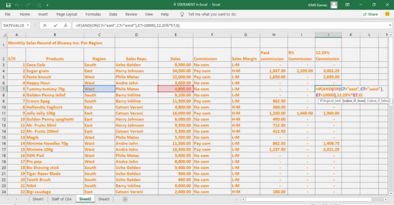
Let us combine the OR, and the AND IF statements in the following example. The management of Bluewy Inc. decided to pay a commission of 12.25% to any of the east or west regions with sales above 10000.
In this case, sales of ABOVE 10000 MUST be made in the East OR West regions. To solve this problem, we do the following:
- The OR function should be as follow: =OR(east, west)
- The AND function should be written thus, =AND(OR(east, west),>10000). This means that if the sales are in either east or west, it must be above 10000.
- Create another column called 12.25% commission, and enter the following formula in cell J3.
- Use the autofill handle to copy the formula to other cells in the column.
- The result of the OR AND IF function is shown below. Take note of who received the commission and who did not receive the commission.
How to Use IF Statements in Excel for Multiple Conditions (IFS function in Excel)
With the nested IF statement, we can test for multiple conditions at the same time. However, this pattern is confusing, especially for beginners. In Microsoft Excel 2019, and Microsoft 365, another function was introduced to remedy the situation. This function is called the IFS function.
The IFS function is used to test multiple conditions at the same time. When used, it will return the value of the first TRUE condition like the nested IF statement. Here, there is no value if false.
When using the IFS function, you are allowed to test up to 127 conditions at the same time. However, it is recommended not to use too many conditions. This is because you are required to enter these conditions in the correct order to avoid mistakes.
For example, in the nested IF statement, you can proceed as follow: <10, <20, <30, etc. If you do anything like <30, <10. <50, you will have the wrong result. Conditions must be entered in the correct order, and this might be difficult to build at times.
Syntax of the IFS function in Excel
The syntax of the IFS function is given by IFS(logical_test1, value_if_true1, [logical_test2, value_if_true2], [logical_test3, value_if_true3],…)
Where:
- logical_test1 is required and is the condition that must evaluate to TRUE or FALSE.
- value_if_true1 is required, and a value that must be evaluated or returned if the condition is TRUE.
- logical_test2 … logical_test127are optional conditions that must evaluate to TRUE or FALSE.
- value_if_true1 … value_if_true127 are optional values or functions that will be evaluated or returned if logical_testn is TRUE.
Example 5: IFS function in Excel
Let’s use the IFS function to grade the students based on their examination scores. We are rewriting the nested IF statement with the IFS function as follows.
- You must have Microsoft Excel 2019 or subscribe to Microsoft 365 to perform this task.
- If you have none of the above, connect to your OneDrive account, and open the Excel app.
- Enter the detail of the students’ results as shown in the worksheet below, using the grades in the nested IF statement.
- Enter the following formula in cell F2: =IFS(E3<40,”F”,E3<50,”E”,E3<60,”D”,E3<70,”C”,E3<80,”B”,E3<=100,”A”)
- Use the autofill handle to copy the formula to other cells in the column.
- Notice that the results of the function are the same as the results of the nested IF statement above. But this function is easier to use than that of the nested IF statement.
Conclusion
The IF statement in excel is very useful when you want to test a condition and output the result. It can be used alongside other logical functions to return a value as have been illustrated in this tutorial.
You can use the nested IF statement in Excel or choose to use the IFS function in Excel. Though the IFS function is easier to use, you must have Microsoft Excel 2019 or Microsoft 365 to use it. If you have none of the above, use your OneDrive account to access the Excel app to use the IFS function.
We used different examples to illustrate how to use the IF statement. If you have any questions, please, do reach out to us. Next week, we shall look at the Vlookup function in Excel.
What are Logical Functions in Excel: AND, OR, NOT, XOR?
Logical functions in Excel are functions that test whether a specified condition is true or false. The result of the logical test will determine whether to evaluate or not to evaluate a function. For example, based on the result of the test, we can evaluate a function, display information, or display TRUE or FALSE.
There are several logical functions in excel, but the most used are the AND, OR, NOT, and XOR functions. In this tutorial, we are going to explore how to use the AND, OR, NOT, and XOR logical functions in Excel.
Logical Functions in Excel
What are logical functions in Excel?
When there is a need to make a decision before evaluating data in Excel, logical functions will be employed. Logical functions in Excel are decision-making tools used to analyze excel data. When it is employed, it tests a cell and returns a value based on the correct decision.
The AND, OR, NOT, and XOR logical functions return a TRUE or FALSE value depending on the decision evaluated. To evaluate a function and return a value, these functions are used alongside the IF function.
For example, the formula: =IF(AND(C3=”South”,D3=”Uche Golden”),”Correct”,”Wrong”) will return CORRECT or WRONG depending on the values of C3 and D3. In this tutorial, we shall discuss how to use the four logical functions displayed in the table below.
Function Detail Example Remark AND Evaluates to TRUE if all arguments are true =AND(C3=”South”,D3=”Uche Golden”) Returns TRUE only if C3 is South and D3 is Uche Golden OR Evaluates to TRUE if any of the arguments are true =OR(C3=”South”,D3=”Uche Golden”) Returns TRUE if C3 is South or D3 is Uche Golden or one of them is true or both of them are true. NOT Evaluates to TRUE if the argument is false, and vice versa =NOT(C3=“South”) Returns TRUE only if C3 is not South. I.e. if C3 is West, it returns TRUE. XOR Evaluates to TRUE only if the argument is an exclusive OR =XOR(C3=”South”,D3=”Uche Golden”) Returns TRUE if C3 is South and D3, not Uche Golden, or if C3 if not South and D3 are Uche Golden. Facts about logical functions in excel
When using the logical functions in Excel, you should attempt to observe the following important facts.
- Microsoft Excel 2003 version and lower accepts up to 30 arguments of a logical function. However, the formula length shall not exceed 1024 characters.
- Microsoft Excel 2007 and higher accepts up to 255 arguments of a logical function. But the formula length shall not exceed 8192 characters.
- Logical functions accept any of the following arguments: Mcrosoft Excel functions, numbers, texts, cell references, Booleans, and comparison operators.
- Logical functions do not evaluate a value but return a Boolean value of TRUE or FALSE.
Using the AND, OR, NOT, and XOR Functions in Excel
The AND, OR, NOT and XOR statements return a TRUE or FALSE value depending on the result of the logical test. They use the following arguments:
AND [=AND(logical1,logical2,logical3,…)] – A TRUE is returned if all the logical values are true else FALSE is returned.
OR [=OR(logical1,logical2,…)] – A TRUE is returned if one or both of the logical values are true else FALSE is returned
NOT [=NOT(Logical)] – A TRUE is returned if the logical value is true else FALSE is returned. A logical value is true when the value is not present in the referenced cell.
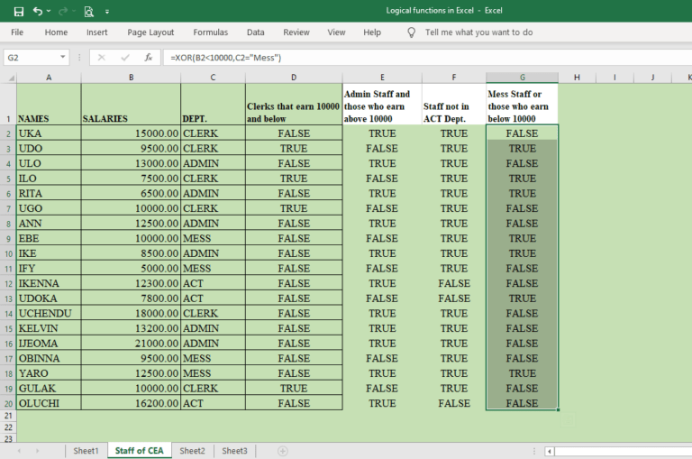
XOR [=XOR(logical1,logical2,…)] – A TRUE is returned if one of the logical values are true else FALSE is returned.
AND function in Excel
The AND function compares more than one condition in the function’s argument. It returns TRUE only if all conditions in the argument are met, and false, if otherwise. This means that when three conditions are specified, the AND returns TRUE if all three conditions are true. If one of the conditions is not true, the AND function returns FALSE.
Let us assume two conditions, A and B in an argument, the AND TRUE table is as follow: =AND(A2=“A”, B2=“B”)
Condition A Condition B AND Value A is true B is true TRUE A is true B is false FALSE A is false B is true FALSE A is false B is false FALSE The syntax of the AND function is given as follow:
=AND(logical1, [logical2],…)
- Where AND is the Microsoft Excel function to be evaluated
- Logical1 is a required argument that must be specified. It is the condition that will be tested and it evaluates to either TRUE or FALSE.
- [logical2] is anoptional argument. When specified, it increases the chances of the argument evaluating to FALSE.
- The optional argument can be increased to up to 254 if the length of the formula is below 8192. Hence, you can have logical3, logical 4, … logicaln.
The AND function in Excel Example
- The table below displays the departments and salaries of different staff of a named organization. Using the AND function, identify the staff in the clerk department whose salary is below 10000.
To solve the above problem, do the following:
- Enter the required data in Excel as shown in the worksheet above.
- Create a column called “Clerks that earn 10000 and below”
- Enter the formula in cell D2, =AND(C2=”Clerk”,B2<=10000)
- Use the autofill handle to fill the formula to other cells below D2.
- The result of the function is displayed below
The function displays TRUE if both conditions, “Clerk” and <=10000 are true, and false if otherwise. You can use the AND function to identify ADMIN staff who earns above 10000.
OR function in Excel
The OR function also compares more than one condition in the function’s argument. It returns TRUE if any of the conditions in the argument are met. It, however, returns FALSE if none of the conditions are met.
This implies that when three conditions are specified, the OR function returns TRUE if any or all three conditions are true. If none of the conditions is true, the OR function returns FALSE.
Let us assume two conditions, A and B in an argument, the OR TRUE table is as follow: =OR(A2=“A”, B2=“B”)
Condition A Condition B OR Value A is true B is true TRUE A is true B is false TRUE A is false B is true TRUE A is false B is false FALSE The OR logical function in Excel returns false only when none of the arguments is true.
The syntax of the OR function is given as follow:
=OR(logical1, [logical2],…)
- Where OR is the Excel function to be evaluated
- Logical1 is a required argument that must be specified. It is the condition that will be tested and it evaluates to either TRUE or FALSE.
- [logical2] is anoptional argument. When specified, it increases the chances of the argument evaluating to TRUE.
- The optional argument can be increased to up to 254 if the length of the formula is below 8192. Hence, you can have logical3, logical 4, … logicaln.
The OR function in Excel Example
- The table below displays the departments and salaries of different staff of a named organization. Using the OR function, identify the staff in the Admin department or those who earn above 10000.
To solve the above problem, do the following:
- Use the same data you used in the AND function example
- Create a new column called “Admin Staff and those who earn above 10000”
- Enter the formula in cell E2, =OR(B2>10000,C2=”Admin”)
- Use the autofill handle to fill the formula to other cells below E2.
The result of the function displays TRUE if any of the conditions are true. Here, if staff is in ADMIN, OR evaluates as TRUE, if the salary is >10000, OR evaluates as TRUE. Also, if staff is admin and salary above 10000, OR evaluates as TRUE. But if staff is not ADMIN, and salary is not above 10000, OR evaluates to FALSE.
NOT function in Excel
The NOT function is used to exclude the values you do not want in a function. It returns the opposite of the logical condition in the function’s argument. For example, if the logical test is TRUE, the NOT function returns a FALSE value and vice versa.
The NOT function has only one argument which can be a text, cell reference, etc. Any value in the argument is excluded when the function is evaluated. For example, =NOT(A2=“Blue”) means every other color except blue.
The NOT TRUE table is as follow: =NOT(A2=“A”)
Condition A OR Value A is true FALSE A is false TRUE The NOT logical function in Excel returns false only when the argument in the function is true.
The syntax of the NOT function is given as follow:
=NOT(logical)
- Where NOT is the Excel function to be evaluated
- logical is a required argument that must be specified. It is the condition that will be tested and it evaluates to either TRUE or FALSE.
The NOT function in Excel Example
- The table below displays the departments and salaries of different staff of a named organization. Using the NOT function, identify the staff that is not in the Accounts department.
To solve the above problem, do the following:
- Use the same data you used in the AND function example
- Create a new column called “Staff not in ACT Dept.”
- Enter the formula in cell F2, =NOT(C2=”Act”)
- Use the autofill handle to fill the formula to other cells below F2.
The result of the function displays TRUE if the condition is false, and FALSE if the condition is true. Here, if staff is in Admin, Clerk, or Messenger, NOT evaluates as TRUE, if staff is in ACT, NOT evaluates to FALSE.
XOR function in Excel
This is called the exclusive OR function. The XOR function is used to compare more than one condition in the function’s argument. It returns TRUE if any of the conditions in the argument is met. It, however, returns FALSE if both or none of the conditions are met.
This implies that when three conditions are specified, the XOR function returns TRUE if any of all three conditions are true. If none or all of the conditions are true, the XOR function returns FALSE.
Let us assume two conditions, A and B in an argument, the XOR TRUE table is as follow: =XOR(A2=“A”, B2=“B”)
Condition A Condition B OR Value A is true B is true FALSE A is true B is false TRUE A is false B is true TRUE A is false B is false FALSE The XOR logical function in Excel returns false only when all or none of the arguments is true.
The syntax of the XOR function is given as follow:
=XOR(logical1, [logical2],…)
- Where XOR is the Excel function to be evaluated
- Logical1 is a required argument that must be specified. It is the condition that will be tested and it evaluates to either TRUE or FALSE.
- [logical2] is anoptional argument. The optional argument can be increased to up to 254 if the length of the formula is below 8192. Hence, you can have logical3, logical 4, … logicaln.
The XOR function in Excel Example
- The table below displays the departments and salaries of different staff of a named organization. Identify those who are exclusively in the Mess department or earns less than 10000.
Let’s use the XOR function to identify those in the Mess dept. or those who earn below 10000.
- Use the same data you used in the AND function example
- Create a new column called “Mess Staff or those who earn below 10000”
- Enter this formula in cell G2, =XOR(B2<10000,C2=”Mess”)
- Use the autofill handle to fill the formula to other cells below G2.
The result of the function displays TRUE if any of the conditions are true. Here, if staff is in Mess and salary 10000 and above, XOR evaluates as TRUE. If salary is <10000 and staff not in Mess dept., XOR evaluates as TRUE. But, if staff is in Mess and salary below 10000, XOR evaluates as FALSE. Also, if staff is not in Mess and salary above 10000, XOR evaluates to FALSE.
Conclusion
Logical functions in Excel are used to test the conditions of an argument whether it is TRUE or FALSE. There are different built-in logical functions in Excel, but the most used ones are AND, OR, NOT, and XOR.
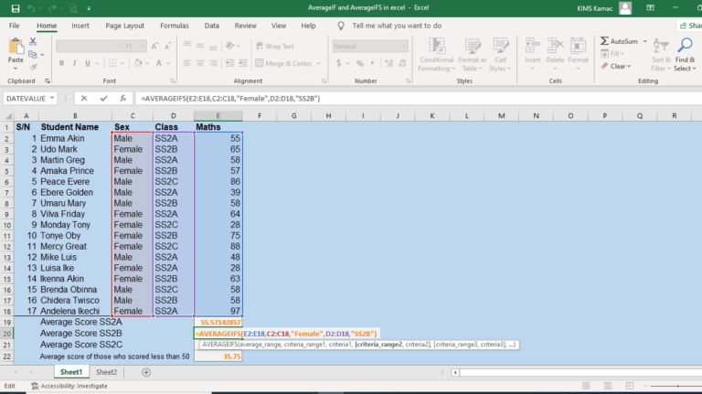
Each of the logical functions evaluates to TRUE or FALSE. To return the actual value, the IF function will be employed.
The AND, OR, and XOR functions compare more than one condition while the NOT function excludes specified conditions.
It is important to master these functions because we shall use them with the IF Statement to return values. Before we continue with the IF Statement in Excel next week, remember to visit our previous tutorials. Don’t forget to share this tutorial with friends.
The AVERAGEIF and AVERAGEIFS Function in Excel
The AVERAGEIF and AVERAGEIFS function in Excel are predefined functions that calculate the arithmetic mean based on specified criteria. You can use either function to calculate the average value of a range of data when they meet specified conditions.
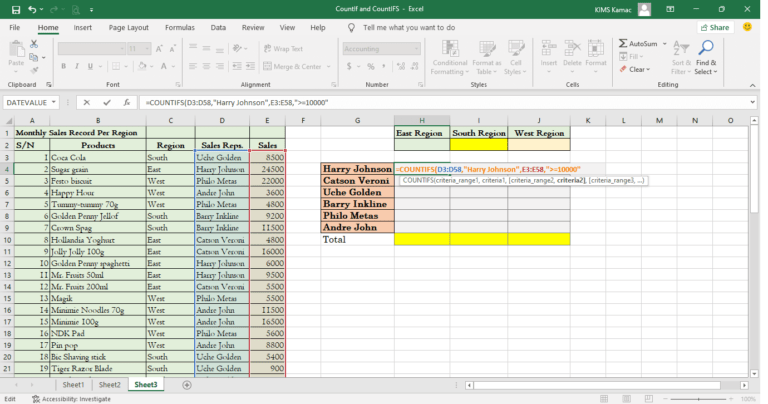
For example, you may want to know the average score of Male students in a class. To evaluate the average score based on the condition (Male students), you will employ the AVERAGEIF function. If there is more than one criterion, you employ the AVERAGEIFS function in Excel.
The AVERAGEIF function is a legacy function while the AVERAGEIFS function was introduced in Microsoft Excel 2007. Both functions are useful when evaluating data that has inherent criteria.
Whereas the AVERAGEIF function accepts one criterion, the AVERAGEIFS function accepts multiple criteria.
In this tutorial, you will learn how to use the AVERAGEIF and AVERAGEIFS function in Excel.
The AVERAGEIF in Excel
The AVERAGEIF in Excel is used to calculate the average or mean values of a range of cells, based on specified criteria. For example, the worksheet below displays the English score of students based on sex and class. To calculate the average score of students in SS2A, you will use the AVERAGEIF function as follow: =AVERAGEIF(D2:D18, “SS2A”, E2:E18)
The above function tells Excel to calculate the average value in the range E2 to E18 if the value in the range D2 to D18 is SS2A. To execute the function, Excel will trace where SS2A appears in column D and select the corresponding value in column E. When all items are selected, they will be summed together and the average value will be calculated.
You can also perform AVERAGEIF in one column only. For example, I can decide to get the mean value of those who scored below 50 in Maths. In this case, it doesn’t matter which class the student belongs to.
To do this, I will execute the following function: =AVERAGEIF(E2:E18,“<50”). In this example, my criterion is less than 50. The output gave a value of 35.75 as shown below.
Notice that only one range was employed in this example (E2:E18), hence, the Average_range was not used. This leads us to the AVERAGEIF syntax.
The AVERAGEIF syntax
The syntax for the AVERAGEIF function is given by: AVERAGEIF(range, criteria, [Average_range])
Where:
- range: is an argument that must be specified (required). This argument represents the range of cells that should specify the AVERAGEIF criteria. See the example above. Such ranges can contain text, numbers, references, and dates.
- criteria: This is also a required argument that must be specified in the function. The criteria can be a number, text, cell reference, or function. It is used to define the cells that average will be calculated. When the criteria specified are met, the average of the corresponding cells will be computed. The criteria argument can accept wild characters such as ? or *.
- The question mark (?) is used to match a single character while the asterisk (*) is used to match a sequence of characters.
- A single character match can be like this, “SS?A”. This will match SS1A, SS2A, SS3A, etc.
- A sequence character match (*) can be represented thus:
- *le: referring to cells that end with le. E.g., female, male, gazelle, etc.
- SS*: referring to cells that begin with SS. E.g., SSS3, SS1B, etc,
- *m*: referring to cells that contain ‘m’. e.g. Amaka, Amara, etc.
- average_range: This is an optional argument in the AVERAGEIF in Excel. This means that this argument may be omitted. However, you can omit it if the average_range is the same as the range argument. Generally, if this argument is omitted, Excel will always compute the argument based on the range argument. But if the range argument is not a number, an error will occur. It is advised that the average_range be the same size and shape as the range argument. If their sizes differ, it might affect the performance of the function.
Example of AVERAGEIF in Excel
The worksheet below displays the sales record of O’ classical Enterprises in three regions: East, West, and South. The general manager wants to know the average sales per region for the month under review. You can use the AVERAGEIF function to analyze the data whereby the regions will form the criteria to compute the average.
The solution can be arrived at by following the following steps:
- Create three columns to represent the East, South, and West regions as shown in the worksheet above.
- Under the east region cell, enter the formula: =AVERAGEIF($C$3:$C$58,”East”,$D$3:$D$58)
- Copy the above formula and paste it into the remaining two cells.
- Under the South cell, change “east” to “south”, and under the West cell, change “east” to “west”.
- Press ENTER after each change to calculate the average.
The AVERAGEIFS in Excel
The AVERAGEIFS function in Excel is used to calculate the mean values of a range of cells, based on more than one criteria. The AVERAGEIFS function can allow up to 127 range/criteria pairs when analyzing data in Microsoft Excel. Unlike the AVERAGEIF function where the range to be calculated appears last, in the AVERAGEIFS, the average_range comes first.
For example, the worksheet below displays the Maths score of students based on sex and class. To calculate the total score of female students in SS2B, I will use the AVERAGEIFS function as follow: =AVERAGEIFS(E2:E18,C2:C18,”Female”,D2:D18,”SS2B”)
The above function tells Microsoft Excel to calculate the average of the values in the range E2 to E18. This average will be calculated if the value in the range C2 to C18 is Female, and the value in D2 to D18 is SS2B. This means that the calculation will be performed only if the Female in columns C matches SS2B in column D.
To execute the function, Excel will trace where Female appears in column C, and where SS2B appears in column D and select the corresponding value in column E. When all items are selected, they will be summed and the average value calculated and displayed.
The AVERAGEIFS syntax
The syntax for the AVERAGEIFS function is given by: AVERAGEIFS(average_range, criteria_range1, criteria1, [criteria_range2, criteria2, … criteria_rangen, criterian])
Where:
- average_range: is an argument that must be specified (required). This argument represents the range of cells that has values for calculating the average value. See the example above. Such ranges should contain numbers.
- Criteria_range1: This is also a required argument that must be specified in the function. The criteria_range1 and criteria1 set up a search pair so that the item in criteria1 will be searched for in criteria_range1. If a match is found, the average calculation takes place, else, the average calculation is omitted.
- criteria1: criteria1 is a required argument. It defines which cells in criteria_range1 that average value will be calculated in the function. The criteria can be a number, text, cell reference, or function. When the criteria specified are met, the mean value will be calculated in the corresponding cells.
- Criteria can accept wild characters such as question mark (?) or asterisk (*). The ? is used to match a single character while * is used to match a sequence of characters.
- A single character match can be like this, “SS?A”. This will match SS1A, SS2A, SS3A, etc.
- A sequence character match (*) can be represented thus:
- *le: referring to cells that end with le. E.g., female, male, gazelle, etc.
- SS*: referring to cells that begin with SS. E.g., SSS3, SS1B, etc,
- *m*: referring to cells that contain ‘m’. e.g. Amaka, Amara, etc.
- criteria_range2, criteria2 … criteria_rangen, criterian: These are optional ranges and criteria up to 127 range/criteria pair. It is used to define the number of range/criteria pairs for the AVERAGEIFS function in Excel. Any of them can be omitted in the function. It is advised that the average_range be the same size and shape as the criteria_range, criteria pair. If their sizes differ, it might affect the performance of the function.
Take note of the following when using the AVERAGEIFS function in Excel:
- Always ensure that text values are in quotation marks when specifying criteria. E.g. “Male”.
- Use wild characters to help match multiple cells, especially, when computing a large set of data.
- Ensure that the average_range contains the same number of columns and rows as the criteria_range argument.
- You can introduce the comparison operators when using the AVERAGEIFS function. For example, =AVERAGEIFS(A2:A10,B2:B10, “>=25”,…)
Example of the AVERAGEIFS function in Excel
The worksheet below displays the sales record of O’ classical Enterprises in three regions: East, West, and South. Each region is controlled by two sales representatives. The general manager wants to know the average sales per Sales Rep. in each region for the month under review.
You can use the AVERAGEIFS function to analyze the data whereby the sales reps and the regions will form the criteria for calculating the average.
Follow the steps highlighted below to solve the above problem.
- Create three columns to represent the East, South, and West regions as illustrated in the worksheet above.
- Create six rows to represent each Sales Rep. in each region as shown in the worksheet above.
- Under Harry Johnson and the East region cell, type in the formula: =AVERAGEIFS($E$3:$E$58,$C$3:$C$58,”East”,$D$3:$D$58,”Harry Johnson”)
- Copy the above formula and paste it under the East region corresponding to Catson Veroni.
- Change the text “Harry Johnson” to “Catson Veroni” and press ENTER.
- Under Uche Golden and the South region cell, type in the formula: =AVERAGEIFS($E$3:$E$58,$C$3:$C$58,”South”,$D$3:$D$58,”Uche Golden”)
- Copy the above formula and paste it under the South region corresponding to Barry Inkline.
- Change the text “Uche Golden” to “Barry Inkline” and press ENTER.
- Copy the above formula and paste it under Philo Metas and the West.
- Change the criteria texts: “South” and “Uche Golden” to “West” and “Philo Metas” respectively. The formula will look like this after the change: =AVERAGEIFS($E$3:$E$58,$C$3:$C$58,”West”,$D$3:$D$58,”Philo Metas”)
- Copy the above formula and paste it under the West region corresponding to Andre John.
- Change the text “Philo Metas” to “Andre John” and press ENTER.
The result shows the average sales of each sales representative and the average sales per region in the period under review. Harry Johnson made the highest average sales while Uche Golden made the least average sales. The East region has the highest average sales while the South region has the least.
Conclusion
The AVERAGEIF and AVERAGEIFS function in Excel are very useful in data analysis. It helps us to compute the mean value based on specified criteria. We can use it to compute templates and distribute them to users for effective data analysis.
The AVERAGEIF function requires one criterion while the AVERAGEIFS require multiple criteria. The major difference in their syntax is that:
- In the AVERAGEIF function, the average_range could be optional and comes as the last argument.
- In the AVERAGEIFS function, the average_range is required and comes as the first argument.
As you have understood how to use these functions, you can start implementing them to relevant data. I will advise you to try as many examples as possible on your own to consolidate your understanding. If you encounter difficulties when applying them to relevant data, reach us through the comment or by contacting us.
Do not forget to check our previous tutorials in this series. Next week, we shall discuss the conditional functions in Excel. Meanwhile, share this with your friends and colleagues.
How to Use the COUNTIFS and COUNTIF Function in Excel
The COUNTIFS and COUNTIF function in Excel are predefined functions that count cells based on specified criteria. You can use either function to count a range of cells when there are conditions associated with your data.
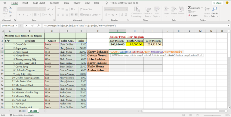
For example, you may want to know the total number of female students in a class. To count the number of students based on the condition (female students), you will employ the COUNTIF function. If there is more than one criterion, you employ the COUNTIFS function.
The COUNTIF function in excel is a legacy function that has been part of the MS Excel 2003 version. But the COUNTIFS function was introduced in MS Excel 2007 and has been useful in counting based on multiple criteria.
While the COUNTIF function accepts one criterion, the COUNTIFS function accepts multiple criteria.
In this tutorial, you will learn how to use the COUNTIFS and COUNTIF functions in Excel.
The COUNTIF Function in Excel
The COUNTIF function in Excel is used to calculate the total number of a range of cells, based on specified criteria. For example, the worksheet below displays the Math score of students based on sex and class. To count the total number of students in SS2A, I will use the COUNTIF function as follow: =COUNTIF(D2:D18, “SS2A”)
The above function states that Excel should count the text in the range D2 to D18 if the text value in the range is SS2A. To execute the function, Excel will count all SS2A that appeared in column D. When all items are selected and counted, the value will be placed in the appropriate cell.
You can also count how many students scored 50 and above in the Math column. To do this, I will execute the following function: =COUNTIF(E2:E18,“>=50”). In this example, my criteria are 50 and above. This leads us to the COUNTIF syntax.
The COUNTIF syntax
The syntax for the COUNTIF function in Excel is given by: COUNTIF(range, criteria)
Where:
- range: is an argument that must be specified (required). This argument represents the range of cells that should specify the COUNTIF criteria. See the example above. Such ranges can contain text, numbers, references, and dates.
- criteria: This is also a required argument that must be specified in the function. The criteria can be a number, text, cell reference, or function. It is used to define the cells that will be counted. When the criteria specified are met, the cells will be counted. Criteria can also accept wild characters such as ? or *. The ? is used to match a single character while * is used to match a sequence of characters. A single character match can be like this, “f?r”. It will match farm, far, Farouk, etc. A sequence character match can be:
- *oon: referring to cells that end with noon. E.g. afternoon, honeymoon, etc
- Good*: referring to cells that begin with good. E.g. good morning, good day, etc,
- *m*: referring to cells that contain ‘m’. e.g. Amaka, Amara, etc.
Example of COUNTIF function in Excel
The worksheet below displays the sales record of Wamco Int’l in three regions: East, West, and South. The general manager wants to know the number of sales made by each sales rep. in the Eastern region for the month under review. You can use the COUNTIF function to analyze the data whereby the Sales Reps will form the criteria for the count.
The solution is given as follow:
There are two sales reps in each region including the Eastern region being evaluated.
- Create two rows to represent the total for each of the eastern sales reps as illustrated in the worksheet above.
- Under Harry Johnson, enter the formula: =COUNTIF(D3:D58,”Harry Johnson”)
- Copy the above formula and paste it under the cell representing Catson Veroni.
- Change “Harry Johnson” to “Catson Veroni” and press ENTER on the keyboard.
From the solution, we observe that Harry Johnson made a total of ten (10) sales in the month under review. However, Catson Veroni made a total of twelve (12) sales. Remember that this solution has nothing to do with the amount of sales made by each sales rep.
The COUNTIFS function in Excel
The COUNTIFS function in Excel is used to count the values in a range of cells, based on more than one criteria. The COUNTIFS function can allow up to 127 range/criteria pairs when analyzing data in Microsoft Excel.
For example, the worksheet below displays the Maths score of students based on sex and class. To count the number of female students in SS2A, I will use the COUNTIFS function as follow: =COUNTIFS(C2:C18,”Female”,D2:D18,”SS2A”)
The above function states that MS Excel should count the values in the range C2 to D18. This count will be evaluated only when the value of C is female and the value of D SS2A. This implies that a female value must have a corresponding SS2A value to be counted, else the count will not execute.
To execute the function, Excel will trace where Female appears in column C, and where SS2A appears in column D and count the corresponding value. When all items are selected, the result will be placed in the selected cell.
The COUNTIFS syntax
The syntax for the COUNTIFS function is given by: COUNTIFS(criteria_range1, criteria1, [criteria_range2, criteria2, … criteria_rangen, criterian])
Where:
- Criteria_range1: This is a required argument that must be specified in the function. The criteria_range1 and criteria1 set up a search pair so that the item in criteria1 will be searched for in criteria_range1. If a match is found, the count takes place, else, the count is omitted.
- criteria1: criteria1 is a required argument. It defines which cells in criteria_range1 will be counted in the function. The criteria can be a number, text, cell reference, or function. When the criteria specified are met, the corresponding cells will be counted. Criteria can accept wild characters such as ? or *. The ? is used to match a single character while * is used to match a sequence of characters. A single character match can be like this, “f?r”. It will match farm, far, Farouk, etc. A sequence character match can be:
- *oon: referring to cells that end with noon. E.g. afternoon, honeymoon, etc
- Good*: referring to cells that begin with good. E.g. good morning, good day, etc,
- *m*: referring to cells that contain ‘m’. e.g. Amaka, Amara, etc.
- criteria_range2, criteria2 … criteria_rangen, criterian: These are optional ranges and criteria up to 127 range/criteria pair. It is used to define the number of range/criteria pairs for the COUNTIFS function. Any of them can be omitted in the function.
Take note of the following when using the COUNTIFS function:
- Always ensure that text values are in quotation marks when specifying criteria. E.g. “Male”.
- Use wild characters to help match multiple cells.
- You can introduce the comparison operators when using the COUNTIFS function. For example, =COUNTIFS(A2:A10, “>=25”,…)
- Each additional range in the argument must have the same number of columns and rows as the criteria_range1 argument.
Example of the SUMIFS function
The worksheet below displays the sales record of Wamco Int’l in three regions: East, West, and South. Each region is controlled by two sales representatives. The general manager wants to know the number of sales that is 10000 and above made by each regional sales rep for the month under review.
You can use the COUNTIFS function to analyze the data whereby the sales reps and the sales will form the criteria for the count.
The solution is given as follow:
There are two sales reps in each region, hence follow the following steps.
- Create three columns to represent the East, South, and West as illustrated in the worksheet above.
- Create six rows to represent each sales rep in each region as shown in the worksheet above.
- Under the east region and the corresponding cell for Harry Johnson, enter the formula: =COUNTIFS($D$3:$D$58,”Harry Johnson”,$E$3:$E$58,”>=10000″)
- Copy the above formula and paste it on the eastern region corresponding to Catson Veroni. Change “Harry Johnson” to “Catson Veroni”.
- Under the south region and the corresponding cell for Uche Golden, enter the formula: =COUNTIFS($D$3:$D$58,”Uche Golden”,$E$3:$E$58,”>=10000″)
- Copy the above formula and paste it on the south region corresponding to Barry Inkline. Change “Uche Golden” to “Barry Inkline”.
- Under the west region and the corresponding cell for Philo Metas, enter the formula: =COUNTIFS($D$3:$D$58,”Philo Metas”,$E$3:$E$58,”>=10000″)
- Copy the above formula and paste it on the west region corresponding to Andre John. Change “Philo Metas” to “Andre John”.
The result shows the total number of sales above 10000 each sales representative was able to achieve in the period under review. Harry Johnson, Philo Metas, and Andre John made the highest number of sales. The southern region made the least number of sales, while Uche Golden did not make any sales 10000 and above.
Conclusion
The COUNTIFS and COUNTIF function in Excel is very useful in data analysis. It helps us to count values based on specified criteria. We can use it to compute templates that will run even in our absence.
The COUNTIF function requires one criterion while the COUNTIFS require multiple criteria.
Haven learned of these functions; you can start implementing them to relevant data. If you encounter difficulties when using them, contact us. Do not forget to check our previous tutorials in this series.
Next week, we shall discuss the AverageIF and AverageIFS functions. Meanwhile, share this with your friends and colleagues.
How to Use the SUMIF and SUMIFS in Excel
The SUMIF and SUMIFS in Excel are predefined functions that calculate totals based on specified criteria. You can either function to manipulate data when there are conditions associated with your data.
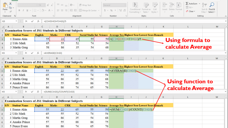
For example, you may want to know the total scores of female students in a class. To evaluate the total based on the condition (male students), you will employ the SUMIF function. If there is more than one criterion, you employ the SUMIFS function.
The SUMIF function is a legacy function that has been part of previous versions of MS Excel. But the SUMIFS function was introduced in MS Excel 2007 and has been useful in evaluating multiple criteria since then.
Whereas the SUMIF function accepts one criterion, the SUMIFS function accepts multiple criteria.
In this tutorial, you will learn how to use the SUMIF and SUMIFS in Excel.
The SUMIF in Excel
The SUMIF in Excel is used to calculate the total values of a range of cells, based on specified criteria. For example, the worksheet below displays the English score of students based on sex and class. To calculate the total score of students in SS2A, I will use the SUMIF function as follow: =SUMIF(D2:D18, “SS2A”, E2:E18)
The above function states that Microsoft Excel should sum the values in the range E2 to E18 if the value in the range D2 to D18 is SS2A. To execute the function, Excel will trace where SS2A appears in column D and select the corresponding value in column E. When all items are selected, they will be summed together to get the total value.
You can also perform SUMIF in one column only. For example, I can decide to sum the values of those who scored below 50 in English. In this case, it doesn’t matter which class the student belongs to.
To do this, I will execute the following function: =SUMIF(E2:E18,“<50”). In this example, my criteria are less than 50. This leads us to the SUMIF syntax.
The SUMIF syntax
The syntax for the SUMIF function is given by: SUMIF(range, criteria, [sum_range])
Where:
- range: is an argument that must be specified (required). This argument represents the range of cells that should specify the SUMIF criteria. See the example above. Such ranges can contain text, numbers, references, and dates.
- criteria: This is also a required argument that must be specified in the function. The criteria can be a number, text, cell reference, or function. It is used to define the cells that will be summed. When the criteria specified are met, the corresponding cells will be added. Criteria can also accept wild characters such as ? or *. The ? is used to match a single character while * is used to match a sequence of characters. A single character match can be like this, “f?r”. It will match farm, far, Farouk, etc. A sequence character match can be:
- *oon: referring to cells that end with noon. E.g. afternoon, honeymoon, etc
- Good*: referring to cells that begin with good. E.g. good morning, good day, etc,
- *m*: referring to cells that contain ‘m’. e.g. Amaka, Amara, etc.
- sum_range: This is an optional argument in the SUMIF function. This means that this argument may be omitted. However, you can omit it if the sum_range is the same as the range argument. Generally, if this argument is omitted, Excel will always compute the argument based on the range argument. But if the range argument is not a number, an error will occur. It is advised that the sum_range be the same size and shape as the range argument. If their sizes differ, it might affect the performance of the function.
Example of SUMIF function
The worksheet below displays the sales record of Wamco Int’l in three regions: East, West, and South. The general manager wants to know the total sales per region for the month under review. You can use the SUMIF function to analyze the data whereby the regions will form the criteria for the sum.
The solution is given as follow:
- Create three columns to represent the total for East, South, and West as illustrated in the worksheet above.
- Under the eastern region cell, enter the formula: =SUMIF($C$3:$C$58,”East”,$D$3:$D$58)
- Copy the above formula and paste it into the remaining two cells.
- Change “east” to “south”, and “east” to “west” respectively.
The SUMIFS in Excel
The SUMIFS in Excel is used to calculate the total values of a range of cells, based on more than one criteria. The SUMIFS function can allow up to 127 range/criteria pairs when analyzing data in Microsoft Excel. Unlike in the SUMIF function where the range to be summed appears last, in the SUMIFS, the sum_range comes first.
For example, the worksheet below displays the Maths score of students based on sex and class. To calculate the total score of female students in SS2A, I will use the SUMIFS function as follow: =SUMIFS(E2:E18,C2:C18,”Female”,D2:D18,”SS2A”)
The above function states that MS Excel should sum the values in the range E2 to E18. This sum will be calculated if the value in the range C2 to C18 is Female, and the value in D2 to D18 is SS2A. This means that the calculation will be performed only if the Female in columns C matches with SS2A in column D.
To execute the function, Excel will trace where Female appears in column C, and where SS2A appears in column D and select the corresponding value in column E. When all items are selected, they will be summed together to get the total value.
The SUMIFS syntax
The syntax for the SUMIFS function is given by: SUMIFS(sum_range, criteria_range1, criteria1, [criteria_range2, criteria2, … criteria_rangen, criterian])
Where:
- sum_range: is an argument that must be specified (required). This argument represents the range of cells that should be summed. See the example above. Such ranges can contain numbers.
- Criteria_range1: This is also a required argument that must be specified in the function. The criteria_range1 and criteria1 set up a search pair so that the item in criteria1 will be searched for in criteria_range1. If a match is found, the sum takes place, else, the sum is omitted.
- criteria1: criteria1 is a required argument. It defines which cells in criteria_range1 will be summed in the function. The criteria can be a number, text, cell reference, or function. When the criteria specified are met, the corresponding cells will be added. Criteria can accept wild characters such as ? or *. The ? is used to match a single character while * is used to match a sequence of characters. A single character match can be like this, “f?r”. It will match farm, far, Farouk, etc. A sequence character match can be:
- *oon: referring to cells that end with noon. E.g. afternoon, honeymoon, etc
- Good*: referring to cells that begin with good. E.g. good morning, good day, etc,
- *m*: referring to cells that contain ‘m’. e.g. Amaka, Amara, etc.
- criteria_range2, criteria2 … criteria_rangen, criterian: These are optional ranges and criteria up to 127 range/criteria pair. It is used to define the number of range/criteria pairs for the SUMIFS function. Any of them can be omitted in the function. It is advised that the sum_range be the same size and shape as the criteria_range, criteria pair. If their sizes differ, it might affect the performance of the function.
Take note of the following when using the SUMIFS function:
- Always ensure that text values are in quotation marks when specifying criteria. E.g. “Male”.
- Use wild characters to help match multiple cells.
- Ensure that the sum_range contains the same number of columns and rows as the criteria_range argument.
- You can introduce the comparison operators when using the SUMIFS function. For example, =SUMIFS(A2:A10,B2:B10, “>=25”,…)
Example of the SUMIFS function
The worksheet below displays the sales record of Wamco Int’l in three regions: East, West, and South. Each region is controlled by two sales representatives. The general manager wants to know the total sales per sales rep. in each region for the month under review.
You can use the SUMIFS function to analyze the data whereby the sales reps and the regions will form the criteria for the sum.
The solution is given as follow:
- Create three columns to represent the total for East, South, and West as illustrated in the worksheet above.
- Create six rows to represent each sales rep in each region as shown in the worksheet above.
- Under the east region and the corresponding cell for Harry Johnson, enter the formula: =SUMIFS($E$3:$E$58,$C$3:$C$58,”East”,$D$3:$D$58,”Harry Johnson”)
- Copy the above formula and paste it on the eastern region corresponding to Catson Veroni. Change “Harry Johnson” to “Catson Veroni”.
- Under the south region and the corresponding cell for Uche Golden, enter the formula: =SUMIFS($E$3:$E$58,$C$3:$C$58,”South”,$D$3:$D$58,”Uche Golden”)
- Copy the above formula and paste it on the south region corresponding to Barry Inkline. Change “Uche Golden” to “Barry Inkline”.
- Under the west region and the corresponding cell for Philo Metas, enter the formula: =SUMIFS($E$3:$E$58,$C$3:$C$58,”West”,$D$3:$D$58,”Philo Metas”)
- Copy the above formula and paste it on the west region corresponding to Andre John. Change “Philo Metas” to “Andre John”.
The result shows the total sales each sales representative was able to achieve in the period under review. Harry Johnson made the highest sales while Uche Golden made the least sales.
Conclusion
The SUMIF and SUMIFS in Excel are very useful in data analysis. It helps us to compute totals based on specified criteria. We can use it to compute templates that will run even in our absence.
The SUMIF function requires one criterion while the SUMIFS require multiple criteria. The major difference in their syntax is that:
- In the SUMIF function, the sum_range could be optional and comes as the last argument.
- In the SUMIFS function, the sum_range is required and comes as the first argument.
Haven learned of these functions; you can start implementing them to relevant data. If you encounter difficulties when using them, contact us.
Do not forget to check our previous tutorials in this series:
- What is Microsoft Excel: Tutorial 1
- Entering and formatting data in Excel: Tutorial 2
- Conditional formatting in Excel: Uses and Applications
- Formatting Numbers and Worksheet in Excel
- What is Cell Referencing in Excel?
- Understanding How to Use Excel Formulas and Functions
Next week, we shall discuss the COUNTIF and COUNTIFS functions. Meanwhile, share this with your friends and colleagues.