Category: InfoComTech

Information technology has changed business processes, information management, information dissemination, and commerce in recent times. Virtually everything we do has a link with technology.
Learn coding and programming the easy way. The knowledge you need to unmask your creativity and creative ability.

  • Understanding How to Use Excel Formulas and Functions

    Understanding How to Use Excel Formulas and Functions

    This tutorial introduces how to use Excel formulas and functions. Formulas are expressions entered by a user for the purpose of calculating cell values. Functions, on the other hand, are predefined formulas built into Excel that assist in data analysis.

    Microsoft Excel has over 450 inbuilt functions, many introduced at different versions of Excel. For example, the VAR.S function was introduced in Excel 2010 while the CONCAT function was introduced in Office 2019. Between 2010 and 2019, over 100 new functions were introduced for effective data analysis.

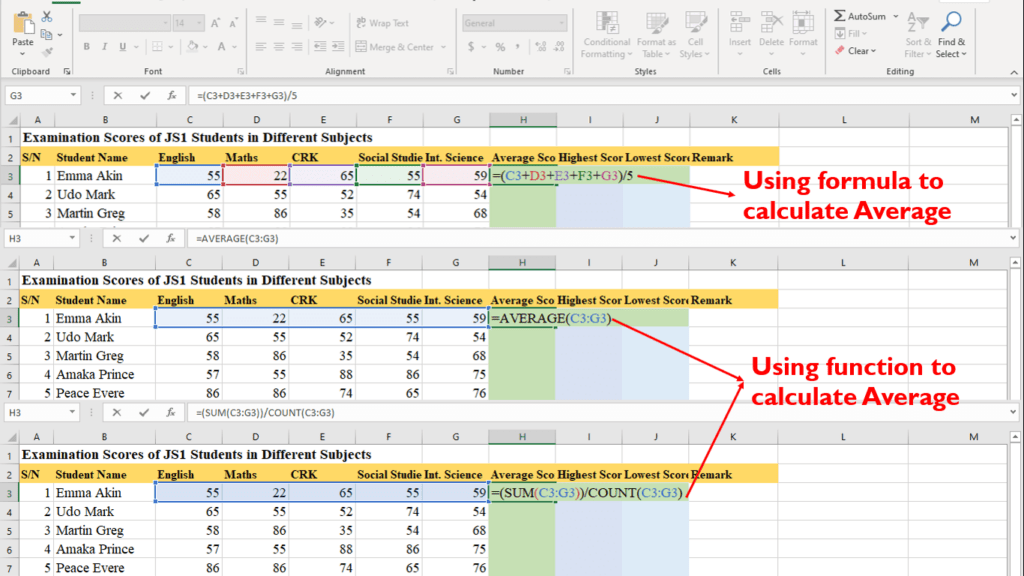
    For example, the worksheet below shows the difference between using a formula and a function in Excel.

    how to use excel formulas and functions

    When a formula is used, cell references are combined with mathematical operators to calculate the value of a cell. But some functions make it easy to perform calculations without introducing mathematical operators.


    In this tutorial, we shall look at how to use Excel formulas and functions in the following headings:

    • What are Excel formulas and functions?
    • Inserting formulas and functions in a worksheet
    • How to use Excel formulas and functions

    What are Excel Formulas and Functions?

    Formulas in Excel

    In Microsoft Excel, formulas are expressions used to manipulate data within a cell or range. Formulas combine mathematical operators with cell references or addresses to determine the value of the selected cell.

    In Microsoft Excel, users can insert different kinds of formulas depending on the calculation required. For example, the following formulas perform different calculations in Excel.

    OperatorFormulaDescription
    +=A2+B2+C2+D2+E2Addition
    =E2-D2Subtraction
    *=B2*C2Multiplication
    /=D2/E2Division
    ^=C2^D2Exponential
    * /=(B2*C2*D2)/100Simple interest

    Formulas are tedious to enter and require carefulness to avoid violating operator precedence.

    Functions in Excel

    Functions are predefined formulas in Excel used to perform operations on data. Using them requires you to reference a cell or range of cells to compute cell values.  There are different kinds of built-in functions in Excel. These functions fall into different categories. Some examples are:

    CategoryFunctionDescription
    FinancialIRRUsed to calculate the internal rate of return
    LogicalANDUsed to check if all arguments are true
    TextUPPERUsed to convert text to capital case
    Date & TimeDAYUsed to return the exact day of the month
    Lookup & ReferenceROWSUsed to return the number of rows in an array
    Math & TrigABSUsed to return the absolute value of a number
    StatisticalAVERAGEUsed to calculate and return the mean of an array
    EngineeringCONVERTUsed to convert a number from a unit to another
    CubeCUBEMEMBERUsed to return a member from connection
    InformationISTEXTUsed to check if a given value is a text or not
    CompatibilityFLOORUsed to round a number down to the nearest level of significance
    WebWEBSERVICEUsed to return data from a web service

    These categories provide users with relevant functions to manipulate and analyze data with ease. However, users need to understand how these functions work in order to use them effectively. One good advantage of a function is that it increases productivity more than using a formula.

    Advance and Basic Excel functions list

    There are a lot of functions in Microsoft Excel that can be used in computation and data analysis. No user can use all these predefined formulas at once.

    There are basic and advanced formulas that are mostly used by users that you can find useful too. Some of the functions appear under the AutoSum category and make calculations easy. Some of these functions include:

    FunctionExampleDescription
    SUM=SUM(B2:B10)Adds up values in the selected range
    AVERAGE=AVERAGE(B2:H2)Computes the average value of the selected range
    COUNT=COUNT(A1:J1)Counts and returns the value of the number of cells that has values within a selected range
    COUNTA=COUNTA(B2:K2)Counts and returns the number of cells that are not empty within a selected range
    MAX=MAX(A1:D1)Computes and returns the maximum value in the selected range
    MIN=MIN(B2:F2)Computes and returns the minimum value in the selected range
    CONCATENATE=CONCATENATE(B2,” “,C2)Used to join text in different cells together
    TRIM=TRIM(C7)Used to remove spaces before or after a text string in selected cells
    ROUND=ROUND(H8,2)Used to round a number to a specified number of digits. The example rounds a number to 2 decimal places.
    IF=IF(H9>50,”Yes”,”No”)Used to check whether a logical condition is true or false and returns the necessary value.
    COUNTIF=COUNTIF(C2:C17,”>50″)Used to count the number of selected cells that meets a specified condition
    SUMIF=SUMIF(C2:C17,”<50″)Used to calculate the sum of values in selected cells that meets a specified condition
    VLOOKUP=VLOOKUP(B20,A2:C11,50,FALSE)Looks for a value in the leftmost column and return a value in the same row from the column you specified

    There are many more functions you will meet as you continue to explore Microsoft Excel. All you need to do is to understand how the function works and use it for your analysis.

    Inserting Formulas and Functions in a Worksheet

    If you must use a formula or function in Excel, you would have to insert the formula in your worksheet.

    To add formula or function in Excel manually, you will need to insert the equal (=) sign first. Typing the (=) equal sign prepares the selected cell to receive formula or function.

    There are five (5) ways you can insert a formula or function in a worksheet, namely:

    1. By manually typing the formula or function. To insert a formula in this manner requires you to type in the (=) sign first. Then the cell reference, followed by necessary operators. When working with a function, after typing the equal sign, follow it by typing the function you want.
    manually insert excel formula
    • You can also use the fx icon on the formula bar. When you click on the icon, a dialog box will appear.
    iuse the insert function dialog
    • On the dialog box that appears enter the function name and click on Go. The list of functionswill appear in the select a function window.
      • Select your desired function and click OK.
      • Another dialog box will appear. The features of the dialog box depend on the selected function.
    what is excel formula
    1. Click on the collapse button to enter the cell references.
      • On the worksheet workspace, select the range of cells and click the collapse button to return to the dialog box.
      • Click OK on the dialog box to calculate the result.
    2. Another way to insert a function is to use the AutoSum dropdown menu on the Home tab, Editing group.
    using autosum

    The dropdown menu has a list of mostly used functions that calculates automatically when selected. However, to display the dialog box as shown in (2) above, select More Functions…   

    1. The fourth way to insert a function in Excel is by using the Insert Function command on the Formula bar. When you select this command, the dialog box as discussed in (2) above will appear.
    subtraction formula in excel
    1. The final way of inserting a function in Excel is by choosing a function from its category on the Formula bar. Choosing any of the functions categories will display the list of functions. Select a function from the list and follow the steps discussed in (2c) above.

    Among these methods of inserting a formula, the manual method will help you work faster and smarter.

    Edit a formula

    While working with a formula, there may be a need for you to edit the formula and make adjustments. When working with Excel formulas and encounter an error, you do not need to delete the formula. You can edit the formula and continue your work.

    To edit a formula,

    1. Select the cell that contains the formula.
    2. Click the formula bar to activate editing (you can also double click the cell)
    3. Make the necessary adjustments and press Enter on the keyboard or click the Enter icon on the formula bar.

    Operator precedence

    When using the manual method to enter formulas in Excel, you should be mindful of the operator precedence. Operator precedence is the sequence by which mathematical operators are executed in an excel formula.

    Microsoft Excel follows the general mathematical rule to carry out its mathematical operations. There are about six (6) arithmetic operators used by excel in formulas. When these operators are used together, the sequence of calculations is what we call operator precedence.

    The operator precedence in Excel is as follows Parenthesis, Exponential, Multiplication and Division, and Addition and Subtraction.

    This order means that whatever is in the parenthesis will be calculated first. Followed by the exponent, then multiplication and division. Addition and subtraction will be performed last in any excel formula.

    For example, in the Excel formula [=C4*D4/E4+F4^2], the multiplication and division will be calculated first. That is, C4*D4/E4. This will be followed by the exponent, that is F4^2, before the addition.

    However, using a parenthesis will change the whole order. For example, if the formula is rewritten thus, [=C4*D4/(E4+F4^2)] the entire result will change. This is because the formula in the bracket will be executed first before other ones.

    How to Use Excel formulas and Functions

    We have already discussed how to insert a formula/ function in excel. However, we shall use the manual method to illustrate how to use Excel formulas.

    Addition and subtraction formula in excel

    The addition formula is used to add values in Excel while the subtraction formula is used to subtract values. Because subtraction represents negative addition, the subtraction function does not exist.

    For example, to subtract the following values: 10 – 2 – 3 – 1 = 10 – (2+3+1). Therefore, to implement subtraction, you can add the negative sign on values. By so doing, adding them will give you the required result.

    In Microsoft Excel, the addition function is called the SUM and it is the simplest function to use in Excel. You can invoke the AutoSum or use the SUM function manually. Let us illustrate below.

    inserting excel formulas
    1. Select the cell you want to calculate addition on
    2. On the Home tab, under Editing, select AutoSum
    3. A range corresponding to the active cell will be automatically selected
    4. If the selected range is correct, press Enter
    5. If the selected range is wrong, use the mouse and select the correct range, and press Enter.

    How to multiply using Excel formula

    The asterisk (*) is used to perform multiplication in Excel. When a formula is entered manually, the asterisk is used to indicate necessary multiplications. For example, B3*C3.

    But, if you are using the excel predefined formula, the multiplication function is called the PRODUCT. To use the PRODUCT function, do the following:

    how to multiply using excel formula
    1. Select the cell you want to calculate multiplication on
    2. On the active cell, enter the (=) sign and start typing product (=PRODUCT)
    3. A list of functions that begin with ‘pro’ will appear.
    4. Select PRODUCT from the list, a parenthesis opens with suggestions for number1, etc.
    5. Enter the cell references to be multiplied separated by a comma.
    6. Close the parenthesis when you are done, and press Enter.

    When working with Excel functions manually, excel provides formula tips that will help you know which value to enter next.

    excel formula tips

    When the first value is entered, separate it with a comma and continue until all the variables are entered.

    Apart from these basic operations, you can use the QUOTIENT function for division and the POWER function for exponent.

    Conclusion

    Excel functions and formulas help us to perform basic and advance calculations in Excel. Formulas can be entered manually by using the predefined functions in Excel.

    Using Excel formulas is easy when you understand how it functions. Whenever you do, pay attention to the formula tips provided by Excel. In our later tutorials, we shall discuss some of the advanced functions in excel, such as the IF, VLOOKUP, etc.

    Our next edition will look at SUMIF and SUMIFS in Excel.

    If you have any questions, please, kindly ask. In case you have not seen our previous tutorials, view them below:

  • What is Cell Referencing in Excel?

    What is Cell Referencing in Excel?

    Cell referencing in Excel is an indispensable knowledge when mastering Microsoft Excel. It is the process of representing the value of a cell in another cell within a workbook.

    Cell references in Excel are a simple way of letting another cell know the value of a cell by using cell addresses. As discussed before, a cell address is represented by the intersection of a column label and a row number.

    For example, the image below shows a worksheet with different cell references for computing students’ total and average scores.

    cell referencing in excel

    In the worksheet above, you can observe that in cell references, you can link to a cell or range. Linking to a cell, e.g., =B1 is the simplest form of a cell reference. In this tutorial, we shall discuss in detail cell referencing in Excel.


    Cell Reference in Excel

    What is a cell reference?

    A cell reference is the value of a cell or range of cells represented in another cell within a worksheet. The cell reference usually represents the address of the referred cell or range in the current cell.

    Because cell referencing copies the value of a cell to another, it is usually used in Excel formulas. They represent a variable in Excel formulas because the result of the formula changes when the value of such cells changes.

    When working with cell referencing in Excel, you can reference cells as follow:

    • Cells within the same worksheet in a workbook
    • Cells in a different worksheet in the same workbook, and
    • Cells in a worksheet in a different workbook

    When cell reference is used in formulas, it helps Excel to locate the actual data or value of such cell. Valid data or values are therefore used by the formula to perform the necessary computations.

    Types of cell reference in excel

    There are three (3) main types of cell reference in Excel, namely

    • Absolute cell reference
    • Relative cell reference, and
    • Mixed cell reference

    There are two (2) other types that are not often used. However, you may find yourself using them in some cases. They are:

    • Circular cell reference, and
    • 3-D cell reference

    Let us discuss each of these types of cell references with examples.

    Absolute cell referencing in excel

    An absolute cell reference is used to represent a constant cell in Microsoft Excel. When working with formulas in Excel, we usually copy and fill formulas into other rows and columns. This helps to save the time it will take to type the same formula in different cells.

    In Microsoft Excel, when formulas are copied, the cell address changes relative to the position of the column/row. This means that, if you copy a formula from cell B2 to cell B3, the reference changes to reflect B3 by default.

    However, in absolute cell referencing, this does not happen. The cell address being copied remains constant across the cells it was copied.

    To achieve absolute cell referencing in Excel, you must add a dollar sign ($) in the cell address. For example, instead of B2, we have $B$2. This will ensure that cell B2 remains constant when it is copied.

    Let us illustrate;

    In the diagram below, if we copy the formula in H2 through H11, the result will be the same as shown.

    absolute cell reference in excel

    What this means is that the value of cell H2 is replicated all through the cells it is copied to. If the value of cell H2 changes, the result in the referenced cells also changes to reflect the change.

    There are cases when you will use absolute cell referencing in computations. For example, if you are working on a variable that has a fixed value, e.g. VAT, interest rate, rent, etc.

    Since the value will remain the same in all computations, it is better to make it constant. If the value changes, it reflects in all computations.

    Relative cell referencing in excel

    Microsoft Excel uses relative cell reference by default. Relative cell referencing is the process of referencing a corresponding cell based on the relative position of a column/row.

    This means that when you copy a formula in cell H2 to cell H3, the cell reference changes to H3. That is, the formula will now refer to the corresponding cells in relation to cell H3.

    This type of cell reference makes working with excel formulas easy and less tedious. Using this type of cell reference, you can copy a single formula to multiple columns/rows and worksheets.

    To use absolute cell referencing, use cell addresses and ranges as they appear by default. That is, use cell A1 as A1 in a referenced cell.

    For example, the diagram below shows that copying the formula in I2 through I11 will vary the result.

    relative cell reference in excel

    The result of cells I2 through I11 will vary depending on the corresponding values of cells in their relative positions. E.g., the value of I5 is the sum of cells C5, D5, E5, F5, and G5.

    The table below shows how relative cell reference works when the autofill handle is dragged downwards.

    example of relative cell references

    Mixed cell referencing in excel

    A mixed cell referencing is a process of keeping the row constant while varying the column and vice versa.

    By default, when a formula is copied down a column, that column becomes constant. Similarly, when copying within the same row, that row becomes constant.

    However, when formulas and functions are copied between rows and columns, you may need to keep either row or column constant.

    A mixed cell reference uses the dollar sign ($) on either the column label or the row number. For instance,

    Mixed Cell ReferenceDescription
    A$1The column is relative while the row is absolute. When copied across columns and rows, values change to reflect the corresponding column position, while rows remain the same.
    $A1The row is relative while the column is absolute. When copied across columns and rows values change to reflect the corresponding row position, while columns remain the same.

    In the example below, we are calculating three (3) different prices of a product based on 3 markups. The price markups appear in row 20 and columns C, D, and E as shown in the worksheet below.

    To get the three price levels for each product, we make the row absolute and make the column relative. And to get the price level of all the products, we make the column absolute and row relative.

    Hence, we enter the following formula in cell D21 [=(1 + C$20)*$C23]. When you drag across columns, you’ll get price 2 and price 3. When you drag across rows, you get prices for each product at each price level as shown below.

    mixed cell referencing in excel

    In the worksheet above, we added the dollar sign (C$20) before the row number to make the row fixed. So, when the formula is copied across the rows, the referenced row remains constant and will not change. Similarly, we added the dollar sign ($C23) before the column label to make the column fixed. So, when the formula is copied across the columns, the referenced column remains constant and will not change.

    Tip: switch between cell references

    You can easily switch between the three types of cell references without typing a dollar sign. To switch between relative to absolute and to mixed cell references, do the following.

    1. Select the cell that contains the cell reference that you want to change, e.g., C2
    2. As the cell is selected, click on the formula bar to activate cell editing
    3. With cell editing active, press F4 on the keyboard.
    4. Continue pressing F4 until you get your desired cell reference type.

    Circular cell referencing in excel

    A circular cell reference is a cell that refers to itself directly or indirectly. Microsoft Excel will usually warn you when you use a circular cell reference, hence it’s not to be advised.

    circular cell references in excel

    However, there are cases when you may use it. For example, in the worksheet above, I entered formula to calculate the cost rate and the cost of a product. The formula is as follow:

    • In cell E2 we have [=F2/D2], to get the product cost rate, and
    • In cell F2 we have [=D2*E2], to get the total product cost

    This is a case of a cell referencing itself indirectly because one value results in another. However, this kind of circular reference is removed when the value of one cell is entered.

    3-d cell referencing in excel

    A 3-d cell reference in excel is used to reference more than one worksheet at the same time. The worksheets to be referenced usually have the same structure.

    For example, the worksheet below calculates the total, average, max, and min scores of students in JS1A, JS1B, and JS1C.

    3d cell references in excel

    The worksheets have the same structure and occupy sheet names: JS1A, JS1B, and JS1C. We want to calculate the summary scores for the 3 classes at the same time in a worksheet. To perform the calculations, we enter the following formulas:

    EnglishMathsAgric.ScienceSocial
    Total score=SUM(JS1A:JS1C!C2:C16)
    Average score=AVERAGE(JS1A:JS1C!C2:C16)
    Max score=MAX(JS1A:JS1C!C2:C16)
    Min score=MIN(JS1A:JS1C!C2:C15)

    The above formula can be easily entered in the required cells as follow:

    1. Select the cell where you want to place the calculation, e.g., B2
    2. Enter the required function, e.g., =SUM(
    3. Select the first sheet tab in the 3d reference, in this case, sheet JS1A
    4. Hold the SHIFT key on the keyboard and click the last sheet tab in the 3d reference, JS1C
    5. Select the data range for the calculation, in this case, C2:C16
    6. Close the bracket and press ENTER on the keyboard.

    Reference cell in excel

    As highlighted above, you can reference a cell within the same worksheet, in a different worksheet and workbook. In this section, we shall look at how to create cell references in excel.

    Reference a cell on the same worksheet

    The examples we have given so far show how to reference a cell on the same worksheet. This can be achieved by referencing a single cell, range, or defined name as shown below.

    Cell ReferenceExplanation
    =C2This is a simple reference that refers to C2 and will return the value of C2 in the selected cell
    =D2:D11This is a range reference that refers to cells D2 through D11. It will return the values of all the cells in the selected range.
    =EngThis is a named reference that refers to a cell or range named ‘Eng’ and will return the value(s) contained in Eng.

    How to create cell reference on the same worksheet

    1. Select the cell in which you want to enter the cell reference.
    2. Type the equal sign (=) on the formula bar. You can also enter the formula you want.
    3. Select a cell or range of cells on the same worksheet.
    referencing a range in same worksheet in excel
    1. If you selected a cell, press Enter key on the keyboard. If you selected a range of cells, hold CTRL+SHIFT and press the ENTER key on the keyboard. You can also close the formula bracket if you entered a formula, and press ENTER on the keyboard.
    2. If you are referencing a defined name,
    referencing a defined name
    1. Type in the defined cell or range name, and press ENTER, or
      1. Press F3 and select the defined name from the Paste Name dialog box, click OK, and press ENTER.

    Reference a cell to another worksheet

    When working with multiple worksheets on the same workbook, you can create cell references between worksheets. The difference between this and the previous is that you will add the sheet name with an exclamation mark (!).

    This can be achieved by referencing a single cell, or range as shown below.

    Cell ReferenceExplanation
    =Sheet1!C2This is a simple cross-reference that refers to Sheet1 and cell C2 and will return the value of C2 in the selected cell
    =Sheet1!D2:D11This is a range cross-reference that refers to Sheet1 and cells D2 through D11. It will return the values of all the cells in the selected range.
    Defined nameDefined names are unique in a workbook. You can refer to a defined name from any worksheet in the same workbook.

    How to create cell reference to another worksheet

    1. Select the cell in which you want to enter the cell reference.
    2. Type the equal sign (=) on the formula bar. You can also enter the formula you want.
    3. Select the sheet tab of the worksheet you want to enter its cell reference.
    4. Select a cell or range of cells in the selected worksheet in (3) above.
    5. If you selected a cell, press Enter key on the keyboard.
      • If you selected a range of cells, hold CTRL+SHIFT and press the ENTER key on the keyboard. You can also close the formula bracket if you entered a formula, and press ENTER on the keyboard.
    referencing another worksheet in same workbook

    Create cell reference to another workbook

    You can also link to a cell, range, or defined name in another workbook. When data in the referenced workbook changes, it updates in the referring workbook as well.

    Here, you will enclose the workbook name in a square bracket followed by the sheet name, and the cell. This can be achieved by referencing a single cell or range as shown below.

    Cell ReferenceExplanation
    ='[workbook name.xlsx]Sheet1′!$G$2Referring to a cell in sheet1 of another workbook
    ='[workbook name.xlsx]Sheet1′!$C$4:$G$4Referring to a range in sheet1 of another workbook
    =’workbook name.xlsx’!definednameReferring to a defined name in another workbook

    How to create cell reference to another workbook

    1. Open both workbooks, if more than two, open all the workbooks.
    2. Select the cell in which you want to enter the cell reference.
    3. Type the equal sign (=) on the formula bar. You can also enter the formula you want.
    4. Select the workbook you want to enter its cell reference.
    5. Select the sheet tab of the worksheet you want to enter its cell reference
    6. If you selected a cell, press Enter key on the keyboard.
      • If you selected a range of cells, hold CTRL+SHIFT and press the ENTER key on the keyboard. You can also close the formula bracket if you entered a formula, and press ENTER on the keyboard.
    7. If you are referencing a defined name,
      • Type in the defined cell or range name, and press ENTER, or
      • Press F3 and select the defined name from the Paste Name dialog box, click OK, and press ENTER.

    Conclusion

    Cell referencing in Excel is very important. Its knowledge will help you master how to add and copy formulas in Excel to make your work easy.

    So far, we have discussed what is cell a cell reference, and the types of cell referencing in Excel. We also discussed how to create cell references in a workbook.

    If you did not understand any part of this tutorial, please, contact us for clarification. We shall continue next week with working with formulas in Excel. Before then, kindly click the share button to share.

    Previous tutorials in this series include:

    1. What is Microsoft Excel: Tutorial 1
    2. Entering and formatting data in Excel: Tutorial 2
    3. Conditional formatting in Excel: Uses and Applications
    4. Formatting Numbers and Worksheet in Excel
  • Formatting Numbers and Worksheet in Excel

    Formatting Numbers and Worksheet in Excel

    A worksheet in Excel is a collection of cells organized in columns and rows as in a table. A worksheet is a workspace where a user enters data and performs the necessary computations on data.

    Worksheet in Excel 2016, is made up of 16384 columns and 1048576 rows with columns labeled from A to XFD.

    Due to the size of an Excel worksheet, it is difficult to use all the cells in a worksheet. However, you can format data, convert a range to a table, print a range and entire worksheet. For example, the worksheet below displays data with different formatting, and a selection to be printed.

    worksheet in excel

    By default, Excel 2016 has one worksheet. You can add more sheets in a workbook, but one worksheet will always be active at a time. Protecting a worksheet restricts users from modifying its content.

    When numeric data is entered in a worksheet, you can format them using available number formats. In this tutorial, we shall discuss how to format numbers and manage worksheets in excel.


    Formatting numbers in Excel

    When you enter numeric data in an Excel worksheet, you have the liberty to format the cells. There are different number formats you can use when formatting numbers in excel. Some of them include currency, percentages, decimals, dates, and phone numbers.

    Number formats

    There are 12 number formatting commands in Excel that you can use to format your cells in a worksheet. They include the following:

    formatting numbers in excel
    1. General: This is the default number format that Excel applies to every data entered in a worksheet, except explicitly specified.
    2. Number: When formatting numbers you can use the number format to indicate a number. If this format is used, you can use a thousand separators and specify the number of decimal places.
    3. Accounting: When used, it displays the currency symbol, a thousand separator, and rounds to 2 decimal places. However, it aligns the currency symbol to the left.
    4. Currency: When used, it displays the currency symbol, a thousand separator, and rounds to 2 decimal places. However, it aligns the currency symbol with the number.
    5. Percentage %: used to multiply a number by 100, and attaching the % sign.
    6. Fraction: Used to display a fractional number.
    7. Scientific: Is used to display a number in exponential notation thus, AE+n. For example, 6580025864 can be displayed as 6.58E+9.
    8. Date: used to format date values of different formats.
    9. Time: used to format time values.
    10. Text: Converts content to text even if it is a number value. Values with the text number format cannot be used for computations.
    11. Special: used to display numbers as zip code, and phone number. Formats are usually displayed in United States patterns.
    12. Custom: Used to modify a number format. You can use it to add a number format of your choice. For detail about custom number formats, visit here.

    Apply a number format to a cell

    1. Select a cell or range of cell
    2. On the Home tab, under the Number group, select the dropdown arrow.
    number formats in excel
    1. Select any of the number formats from the list
    2. It will be applied automatically to the selected cell or range.

    You can also, apply formatting to numbers by invoking the number dialog box. To open the dialog box, do any of the following:

    1. Press CTRL+1 on the keyboard, and select the Number tab.
    2. Click the number dialog box launcher on the Number group.
    3. From the dropdown list on the Number group, select More Number Formats…
    4. Right-click a cell or range of cells and select Format Cells… from the popup list
    formatting cells
    1. On the Home tab, under Cells, select Format. From the dropdown list, select Format Cells
    cell formatting with number formats
    1. When the dialog box appears, select the Number tab.
    select a number format
    1. On the dialog box, choose a number format and the necessary features you want.
    2. When done, click OK.

    Managing worksheets in Excel

    Managing worksheet in Excel includes modifying worksheets for ease of use and access. You can insert, rename, copy or delete a worksheet in excel.

    Insert a Worksheet

    Microsoft Excel 2016 has one worksheet by default. To include more than one worksheet in a workbook, you will need to insert more sheets. To insert a worksheet, do any of the following:

    • On the base of the Sheet, select the (+) icon to the right of the last sheet in a workbook.
    • On the Home tab, under Cells, select Insert. From the list, select Insert Sheet.
    • Right-click an existing worksheet. From the popup list, select Insert. Select Worksheet on the dialog box that appears, and click OK.
    inserting a worksheet in excel

    Rename a worksheet

    To rename a worksheet, do any of the following:

    • Double-click the sheet you want to rename. When the name is selected, delete the existing name and type a name of your choice.
    • Right-click the sheet you want to rename. Select Rename from the popup list. Rename the selected sheet.

    Delete a worksheet

    To delete a worksheet, do any of the following:

    • Right-click the sheet you want to delete. Select Delete from the popup list. Select Delete from the dialog box that appears.
    • On the Home tab, under Cells, select Delete. From the list, select Delete Sheet.

    NB: If the sheet you are deleting does not have content, the sheet will be deleted outrightly. If the sheet has content, a dialog box will notify you that all the content will be permanently deleted.

    Move or copy a worksheet

    To move a worksheet, select and drag the worksheet tab to any tab location of your choice.

    To copy a worksheet, do the following:

    1. Hold the CTRL key and drag the worksheet tab to a tab location of your choice.
    2. Right-click the worksheet you want to copy.
      1. From the popup list that appears, select Move or copy
    copy a worksheet in excel
    1. From the dialog box that appears, select the Create a copy check box
      • Under Before sheet, select where you want to place the copy of the sheet.
      • Click OK when done.

    Hide/unhide a worksheet

    If you want to hide a worksheet, do any of the following:

    1. Right-click the sheet you want to hide, and select Hide from the popup list. The sheet will be automatically hidden.
    2. On the Home tab, under the Cells group, select Format
    hide sheets in excel
    1. From the format dropdown list, point to Hide & Unhide and select Hide Sheet.
    2. The selected sheet will be hidden.

    To unhide a worksheet, do the following:

    1. Right-click any worksheet tab, and select Unhide from the popup list.
    2. On the Home tab, under the Cells group, select Format.
      • From the format dropdown list, point to Hide & Unhide and select Unhide Sheet.
    3. In either case, a dialog box will appear.
    select to unhide worksheets
    1. On the dialog box, select the sheet you want to unhide and click OK.
    2. The selected worksheet will appear.

    Grouping Worksheets in Excel

    When you need to perform the same action in more than one worksheet, it’s easier to group them. Grouped worksheets make it easier to enter the same data in more than one worksheet at the same time.

    For example, you can do any of the following, and more in a grouped worksheet.

    • Enter the same data/ formula/ formatting in more than one worksheet at the same time
    • Perform the same calculation in more than one worksheet
    • Move, copy or delete more than one worksheet
    • Print selected worksheets
    • Correct similar typographic error in more than one worksheet

    Grouping worksheets will help you save time and eliminate redundant data entry.

    Group worksheets together

    To group a worksheet, the worksheets should have similar structures. Do the following to group worksheets:

    1. Press and hold the CTRL key on the keyboard, and select the worksheets you want to group together
    2. If the sheets are together, then, select the first sheet, hold the SHIFT key, and select the last sheet.
    3. Start modifying the worksheets.
    group worksheets in excel
    1. All changes will take place in all grouped worksheets at the same time.

    Move or copy a grouped worksheet

    You can move a grouped worksheet by:

    1. Clicking on a tab on the grouped worksheet
    2. Drag the group to any tab location of your choice

    To copy grouped worksheets:

    1. Right-click any of the grouped worksheets you want to copy.
    2. From the popup list that appears, select Move or Copy
    3. From the dialog box that appears, select the Create a copy check box
    4. Under Before sheet, select where you want to place the copy of the grouped worksheets.
    5. Click OK when done.
    6. The sheets are automatically copied to the chosen location.

    Ungroup selected worksheets

    To ungroup selected worksheets:

    1. Hold the CTRL key and select the sheet you want to ungroup.
    2. To ungroup all grouped sheets, simply click on one of the sheets that are not grouped.

    Group all worksheets in a workbook

    1. Right-click on one of the sheets tab.
    2. From the popup list, select Select All Sheets
    3. NB: When you group all worksheets, you can ungroup them by clicking on any of the sheets’ tabs. Hence, you cannot browse through the sheets when you grouped all worksheets. However, you can browse through grouped worksheets, if all sheets in a workbook are not grouped.
    4. Youcan also ungroup all worksheets by right-clicking a sheet, from the popup list, select Ungroup Sheets.

    Deleting a grouped worksheet

    • Right-click the grouped worksheet you want to delete. Select Delete from the popup list. Select Delete from the dialog box that appears.
    • On the Home tab, under Cells, select Delete. From the list, select Delete Sheet.

    Hiding grouped worksheets

    If you want to hide a grouped worksheet, do any of the following:

    1. Right-click the grouped sheet you want to hide, and select Hide from the popup list. The grouped worksheets will be automatically hidden.
    2. On the Home tab, under the Cells group, select Format
      • From the format dropdown list, point to Hide & Unhide and select Hide Sheet.
      • The selected sheets will be hidden.

    Unhiding grouped worksheets

    To unhide hidden grouped worksheets, do the following:

    1. Right-click any worksheet tab, and select Unhide from the popup list.
    2. On the Home tab, under the Cells group, select Format.
      • From the format dropdown list, point to Hide & Unhide and select Unhide Sheet.
    3. In either case, a dialog box will appear.
    4. On the dialog box, select the sheet you want to unhide and click OK.
    5. Repeat the same process until you are done.

    Modifying Columns and Rows in Excel

    As earlier discussed, the worksheet in Excel is made up of rows and columns. Columns are vertical cells that run from up to down. They have a column label that begins with A and ends in XFD.

    Similarly, rows are horizontal cells that run from left to right. They have row numbers that begin with 1 and end in 1048576.

    Both columns and rows play an important role in a worksheet because their combination gives birth to a cell. Also, the column label and row number are used as a reference or an address for every selected cell.

    When working on a worksheet, there are columns and rows modifications that are necessary for effective management. In this section, we shall discuss how to insert, delete, hide and resize columns and rows in Excel.

    Inserting and Deleting Columns and Rows

    Assuming you are working on a worksheet, and there is a need for you to add a column or row. For example, in the worksheet below, I want to add a column before Watts and a row before Fridge.

    inserting rows and columns

    To achieve this, do the following:

    To insert a column:

    1. On the worksheet, select a cell on column C or the entire C column.
    2. On the Home tab, under the Cells group, select Insert.
    3. From the dropdown menu, select Insert Sheet Columns.
    4. The column will be added, shifting the Watts column to the right. Hence, the new column becomes column C.
    5. You can also, right-click on top of the Column C label. From the popup list, select Insert.

    To Insert a row:

    1. On the worksheet, select a cell on row 6 or the entire Row 6.
    2. On the Home tab, under the Cells group, select Insert.
    3. From the dropdown menu, select Insert Sheet Rows.
    4. The row will be added, shifting Fridge Row down. Hence, the new row becomes row 6.
    5. You can also, right-click on the row number “6”. From the popup list, select Insert.

    The output of the above exercise is shown in the image below.

    insert a new column and row

    To delete a column/ row,

    1. On the worksheet, select the columns or rows you want to delete or a range within the columns/ rows
    2. Go to Home, under Cells, select Delete
    3. From the dropdown menu that appears, select either Delete Sheet Columns or Delete Sheet Rows
    4. The columns or rows will be automatically deleted.

    Inserting Multiple Columns & Rows

    To insert more than one column or row in a worksheet, do the following.

    For columns:

    1. Highlight the number of columns you want to insert beginning from the insertion point, e.g., 4 columns
    2. Hold down the SHIFT or CTRL key on the keyboard.
    3. With the CTRL or SHIFT pressed, right-click one of the selected column labels
    4. From the dropdown menu, select Insert.
    5. The exact number of highlighted columns will be inserted, moving other columns to the right.

    For rows:

    1. Highlight the number of rows you want to insert beginning from the insertion point, e.g., 3 rows
    2. Hold down the SHIFT or CTRL key on the keyboard.
    3. With the CTRL or SHIFT pressed, right-click one of the selected row numbers
    4. From the dropdown menu, select Insert.
    5. The exact number of highlighted rows will be inserted, moving other rows down.

    TIP: If the selected column or row has formatting applied, the new column/ row will inherit the formatting. To remove the formatting, select the Insert Options button on the inserted column/ row, and select Clear Formatting.

    insert options in new columns/ rows

    Inserting & Deleting Cells

    To insert cells,

    1. Select the cell or range where you want to insert cell(s)
    2. Right-click the selected cell(s), from the popup menu, select Insert
    3. A dialog box appears
    insert cells
    1. On the dialog box, choose either Shift cells right or Shift cells down.
    2. You can also go to Home > Cells > Insert > Insert Cells...

    To Delete a cell,

    1. Select the cell or range you want to delete
    2. Right-click the selected cell(s), from the popup menu, select Delete
    3. A dialog box appears
    4. On the dialog box, choose either Shift cells left or Shift cells up.
    5. You can also go to Home > Cells > Delete > Delete Cells...

    Modifying cell width and height

    To adjust column width,

    1. Place the pointer on the line that divides two columns, the pointer changes to a cross.
    2. Click and drag to the left (to reduce width) or to the right (to expand width)
    modifying cell height and width

    You can also, adjust more than one column at the same time and with equal width by,

    1. Select the cell, or range, or columns you want to adjust their width
    2. Go to Home, under Cells, select Format
    3. From the format, cells drop-down menu, select Column Width…
    resize multiple columns/ rows at the same time
    1. A dialog box appears, enter a width size, and press OK.
    2. You can also choose AutoFit Column Width to fit columns according to the content width.

    To adjust row height,

    1. Place the pointer on the line that divides the two-row numbers, the pointer changes to a cross.
    2. Click and drag to up (to reduce height) or to down (to expand height)

    You can also, adjust more than one row at the same time and with equal height by,

    1. Select the cell, or range, or rows you want to adjust their height
    2. Go to Home, under Cells, select Format
    3. From the format, cells drop-down menu, select Row Height…
    4. A dialog box appears, enter a height size, and press OK.

    Hiding and Unhiding Rows and Columns

    If you want to hide a column or row, do the following:

    To hide column/ row

    1. Highlight the columns/ rows you want to hide
    2. Right-click the column label or row number, and select Hide from the popup list.
    hide a column or row
    1. The sheet will be automatically hidden.
    2. OR, On the Home tab, under the Cells group, select Format
      • From the format dropdown list, point to Hide & Unhide and select either Hide Rows or Hide Columns.
      • The selected column/ row will be hidden.

    To unhide column/ row:

    When you hide a column or a row, a double line appears where there is a hidden column/ row.

    show hidden columns/ rows

    To unhide a column/ row do any of the following:

    1. If only one column/ row was hidden, then, place the pointer on the double line and double-click. The hidden column/row will appear.
    2. If more than one column/ row is hidden,
      • Select adjacent columns/ rows between the hidden columns/ rows
      • On the Home tab, under the Cells group, select Format.
      • From the format dropdown list, point to Hide & Unhide and select Unhide Columns or Unhide Rows
    3. All hidden columns/ rows will appear.

    Conclusion

    Thank you for staying with me till the end of this tutorial. In case you have further questions please, contact us as soon as possible.

    Today’s tutorial centered on working with a worksheet in Excel. We looked at formatting numbers, managing worksheets, and modifying rows and columns in Excel.

    Please, do not forget to visit the previous tutorials in Microsoft Word and Excel, in case you missed them:


    1. What is Microsoft Excel: Tutorial 1
    2. Entering and formatting data in Excel: Tutorial 2
    3. Conditional formatting in Excel: Uses and Applications

    1. What is Microsoft Word: A Practical Overview
    2. How to Create a Document in Microsoft Word
    3. The Page Layout: Microsoft Word Tutorials 3

    If this tutorial has helped you, kindly share it with friends and colleagues. Next week we shall look at What is cell referencing in Excel.

  • Conditional formatting in Excel: Uses and Applications

    Conditional formatting in Excel: Uses and Applications

    Conditional formatting in Excel is an important tool used for effective data analysis. It is a tool that helps you identify and critically visualize cells that have patterns and trends using colors.

    Conditional formatting in Excel helps you to visualize and understand data in a worksheet without the use of charts. It is a tool that incorporates color scales, data bars, and icon set to identify variations in data patterns.

    It is an interesting data analysis tool that identifies cell variations based on true data conditions. When conditions are specified, cells appearances may vary in compliance with the specified conditions.

    For example, the table below displays a household’s monthly electricity consumption in 6 months. Electrical appliances that consumed lower units of electricity are highlighted with light-blue color. As the units increase, the cell color becomes dark yellow. But the appliances with greater units are highlighted with green color.

    conditional formatting in Excel

    Notice that the total row, in the table above, used an icon set to show deviations from the base value. Values higher than the base value are indicated with an up-level icon. Similarly, lower values are identified with a down-level icon.

    In this tutorial, we discussed what is conditional formatting in Excel and how to use them in your datasets.


    Previous Excel Tutorials:


    What is Conditional Formatting in Excel?

    Conditional formatting in Excel is a tool that works like a chart. But instead of representing data in the vertical and horizontal axis, data values are represented with colors, bars, and icon sets.

    In Excel, conditional formatting helps the audience to visualize data with clarity and precision without requiring further analysis.

    For example, in the table above, one will easily observe the 3 electrical appliances that consume electricity units. These appliances were indicated with the green color as refrigerator, hot plate, and air conditioner.

    Hence, to reduce the total electricity units consumed in a month, the household can reduce the usage of these appliances.

    Thus, conditional formatting in excel is a command that helps you to identify variations in data values within a selected range. It allows you to use color scales, data bars, and icon sets to highlight data values for a clearer understanding.

    Uses of conditional formatting in Excel

    At what point would you use the conditional formatting in excel? Or what are the benefits or usefulness of conditional formatting in excel? From experience and usage, we can identify the following benefits of conditional formatting.

    1. Conditional formatting is a mini-chart that helps you summarize data at a glance without the use of complex analysis tools. Important values can be easily identified using colors, bars, and icons.
    2. It can help you detect critical issues or set trigger points within a dataset. For example, if you don’t want to spend beyond a particular amount, you can use conditional formatting to set trigger. This alert can be activated with different colors at different data values, say, at 50%, 75%, and 95%.
    3. You can use it to identify unusual values. For example, monthly product sales should not be below the breakeven quantity. You can use conditional formatting to detect when such a scenario occurs.
    4. It is also useful when evaluating formulas to arrive at a solution. For example, you can include a condition using a formula that evaluates to true or false.

    How to copy conditional formatting in excel

    You can copy the conditional formatting in a particular dataset and apply it to another dataset in Excel. You can do this using the format painter.

    To copy conditional formatting, you should make sure that the two datasets are similar. You should not copy the conditional formatting of text-based data to numeric data.

    Do the following when copying conditional formatting in excel.

    1. Locate the conditional formatting of data you want to copy and highlight the cell or range of cells.
    2. On the Home tab, under the Clipboard group, select the Format Painter.
    3. Locate the data where you want to apply the copied conditional formatting on.
    4. Using the format painter pointer, select the cell or range of cells you want to apply the formatting on.
    5. The conditional formatting is automatically applied to the selected cells.

    The quick analysis button

    The quick analysis button in the Excel worksheet helps you to quickly apply formatting to your data. Whenever you highlight data in a cell or range of cells, the quick analysis button appears.

    You can use this tool to apply conditional formatting instead of visiting the Home tab >> Styles group. With the quick analysis tool, you can add charts, tables, totals, and spikelines to selected data.

    To use the quick analysis tool to apply formatting, do the following:

    1. Select the data that you want to apply formatting to or data you want to analyze.
    2. The quick analysis button appears at the lower right corner of the selected items.
    what is conditional formatting
    1. Click the quick analysis button to reveal the different analysis tools you can apply to the selected data.
    2. To apply conditional formatting, select the Formatting tab, and choose any of the conditional formatting options.

    How To Use Conditional Formatting In Excel

    There are five simple ways to use conditional formatting in Excel. They include:

    • Highlight cells rules
    • Create top/bottom rules
    • Use of data bars
    • Selecting color scales, and
    • Specifying icon set

    Highlight cells rules

    This type of conditional formatting is used to identify cells based on preset rules. There are 7 preset rules to be chosen from. They include: greater than, less than, between, equal to, the text contains, date occurs, and duplicate values.

    When a cell meets the given criteria, the specified color is highlighted on such cell. To apply this type of conditional formatting, do the following:

    1. Highlight the cell or range of cells you want to apply conditional formatting on.
    2. On the Home tab, under Styles, select Conditional Formatting.
    how to use conditional formatting in excel
    1. From the dropdown menu, point to Highlight Cells Rules and select Greater than… Note:You can select any of theoptions available depending on the rule you want to set. For example, if you are setting a less than rule, select Less than…
    2. A dialog box appears.
    applying conditional formatting in excel
    1. On the dialog box, specify the greater than value in the text box.
    2. Then select the type of highlight for cells greater than the specified values in the With dropdown box. Notice the effect on the selected cells.
    3. Click OK when done. The specified formatting will be automatically applied.

    You can also use this method to highlight cells which has a particular text value. Also, cells that have values between two values can be identified, and cells with duplicate values.


    Create top/bottom rules

    This type of conditional formatting can be used to set targets and cutoff points in data. For example, in an academic section, we can set a target for top and least performing students.

    Let us assume that the average student scores 55% in the overall assessment. Using the top/bottom rule, we can identify students that scored above average or those that scored below average.

    To use the top/bottom rule, do the following:

    1. Highlight the cell or range of cells you want to apply conditional formatting on.
    2. On the Home tab, under Styles, select Conditional Formatting.
    3. From the dropdown menu, point to Top/Bottom Rules and select Top 10%… Note:You can select any of theoptions available depending on the rule you want to set.
    4. A dialog box appears.
    5. On the dialog box, specify the top% value you want, e.g. 10 or 20, etc, in the text box.
    6. Then select the type of fill for cells that meet the criteria in the With box.
    7. Click OK when done. The specified formatting will be automatically applied.

    You can also use this option to identify values above or below average, and top 10 or bottom 10 values.

    Use of data bars

    A data bar is used to compare values in selected cells or ranges. When a data bar is used, the length of the bars depicts the value in a cell. Higher values have longer bars while lower values have shorter bars.

    Data bars can also be used to specify negative and positive values in a range of cells. Data bars with negative values will extend leftwards, while positive values extend rightwards. However, you should configure the data bars to start from the middle of the cells.

    To apply data bars conditional formatting in Excel, do the following:

    1. Highlight the cell or range of cells you want to apply conditional formatting on.
    2. On the Home tab, under Styles, select Conditional Formatting.
    3. From the dropdown menu, point to Data bars and select any of the preset data bars.
    applying data bars
    1. The specified formatting will be automatically applied to the selected cells.

    You can choose between Gradient Fill and Solid Fill. You can also specify your own rules by clicking the More Rules… When you choose the More Rules button, you will be able to set up your own conditional formatting rules.

    If you selected the More rules option, then do the following:

    1. The New Formatting Rule dialog box will appear.
    managing conditional formatting rules
    1. On the dialog box that appears, under Bar Appearance: change the Solid Fill to Gradient Fill. Choose a color of your choice. I chose a green color.
    2. Select the Negative Value and Axis… button. A dialog box will appear.
    applying negative values in conditional formatting
    1. On the dialog box, leave the negative bar fill color as red. Change the Axis settings to Cell midpoint.
    2. Click OK.
    3. Click OK on the New Formatting Rule dialog box.
    4. The rule will be automatically applied as shown below.
    how to copy conditional formatting in excel

    Selecting color scales

    Color scales are visual guides that perform a similar function as the data bars. The difference is that color scales use color gradations and variations to interpret the difference between two values.

    There are two types of color scales: two-color and three-color scales. Color scale usually compares lower and higher values by using color variations.

    In a two-color scale, lower values are represented with color, e.g., blue, and the higher values with green. Values between the low and high values transform from blue to green depending on the value.

    On a three-color scale, you can represent low, middle, and high values with three different colors. These colors will keep varying depending on the value of a cell with high values shading the high color.

    To use the color scale conditional formatting in excel, do the following:

    1. Highlight the cell or range of cells you want to apply conditional formatting on.
    2. On the Home tab, under Styles, select Conditional Formatting.
    3. From the dropdown menu, point to Color Scales and select any of the preset color scales.
    4. The color scale will be automatically applied to the selected range.
    5. If you selected the More Rules… option, then do the following:
    6. The New Formatting Rule dialog box will appear.
    applying color scales
    1. On the dialog box that appears, under Format Style: choose either two-color or three-color scale.
    2. Choose a color for the minimum value, and the maximum value respectively.
    3. Click OK when done. The rule will be automatically applied.

    Specifying icon set

    The icon set is used to classify values. Each category is separated by a value or range of values. There is different icon set, and you can customize your own icon set. Each of the icons in the set represents lower, middle, and upper values.

    To use icon set in conditional formatting, do the following:

    1. Highlight the cell or range of cells you want to apply conditional formatting on.
    2. On the Home tab, under Styles, select Conditional Formatting.
    3. From the dropdown menu, point to Icon Sets and select any of the preset icon sets.
    choosing icon sets
    1. The selected icon set will be automatically applied to the selected range.
    2. If you selected the More Rules… option, then do the following:
    3. The New Formatting Rule dialog box will appear.
    customizing icon sets in excel formatting
    1. On the dialog box that appears, under Icon Style: choose any of the icons set from the list.
    2. Under Icon, represent each icon based on the anticipated cell value or range of value. You can also change the icon if you want.
    3. Click OK when done. The rule will be automatically applied.

    Conditional formatting in excel formula

    You can use a formula to determine how a cell or range of cells will be formatted. Conditional formatting in Excel formula requires that you specify a logical condition that must evaluate to TRUE/FALSE.

    The true value is represented with 1 and the false value is represented with 0 in the function. For example, we will use a formula to highlight cells that have their margin greater than or equal to 650.

    To apply conditional formatting using Excel formula, do the following:

    1. Highlight the cell or range of cells you want to apply conditional formatting on.
    2. On the Home tab, under Styles, select Conditional Formatting.
    3. From the dropdown menu, select New Rule… The New Rule dialog box will appear.
    consitional formatting in excel formula
    1. On the dialog box, under Select a Rule Type, select Use a formula to determine which cells to format.
    2. In the text box, enter a formula that evaluates to true/false. E.g., [=ISEVEN(A2); =IF(H2>=650,1); =IF(AND(E2<=3000,H2>=400),1), etc.]
    3. Select the Format… button and choose a color of your choice.
    4. Click OK to return to the new rule dialog box.
    5. Click OK to apply the specified rule. The rule is automatically applied.

    Conditional formatting in excel based on another cell

    You can also use conditional formatting to format a cell based on the value of another cell. For example, we shall use conditional formatting to select the products which cost is less than 5000, and whose margin is greater than or equal to 500.

    Do the following:

    1. Highlight the cell or range of cells you want to apply conditional formatting on.
    2. On the Home tab, under Styles, select Conditional Formatting.
    3. From the dropdown menu, select New Rule… The New Rule dialog box will appear.
    4. On the dialog box, under Select a Rule Type, select Use a formula to determine which cells to format.
    5. In the text box, enter the formula [=IF(AND(E2<=5000,H2>=500),1)]
    6. Select the Format… button and choose a yellow color.
    7. Click OK, then click OK. The cells that meet the condition will be automatically selected as shown below.

    Clear Conditional Formatting in Excel

    To remove conditional formatting in Excel, do the following:

    1. Highlight the cell or range of cells you want to remove conditional formatting on.
    2. On the Home tab, under Styles, select Conditional Formatting.
    3. From the dropdown menu, point to Clear Rules…
    4. From the list that appears, select either:
      • Clear Rules from Entire Sheet (clears all rules in the worksheet)
      • Clear Rules from Selected Cells (Clears all rules in the selected cells)

    Conclusion

    Conditional formatting in Excel is an interesting tool that helps you quickly summarize and analyze data. It is easy to apply and it visualizes data for clarity and ease of comprehension.

    We discussed in this tutorial, what is conditional formatting in Excel. Here we discussed conditional formatting and its uses.

    We further looked at how to use conditional formatting in Excel. Here we identified five ways of applying conditional formatting with examples.

    We finally looked at how you can use a formula to apply conditional formatting. There are few things we did not cover: managing rules in conditional formatting. If you have a question regarding this, please, indicate it in the comment section. Next week we shall continue with formatting numbers and worksheets in Excel.

  • Entering and formatting data in Excel: Tutorial 2

    Entering and formatting data in Excel: Tutorial 2

    Entering data in Excel is the same as typing text and numbers into the cells in an Excel worksheet. Formatting data in Excel is a process of modifying and customizing the texts and numbers entered.

    As discussed in Microsoft Excel Tutorial 1, a cell is an intersection between a column label and a row number. This box has a reference or an address that is referred to when performing computations and analysis.

    Before we can analyze or compute data in MS Excel, we must first enter the necessary data row-wise or column-wise. Depending on the nature of the analysis, formatting data and cells may be necessary.

    In this tutorial, we shall look at how to enter and format data in an excel worksheet.


    Entering Data in Excel

    Entering data in Microsoft Excel can be done in three major ways:

    1. By typing in data into individual cells in an Excel worksheet,
    2. By copying and pasting data from another source to selected cells in a worksheet
    3. By importing data from an external data source

    Enter data in a row or column

    Microsoft Excel workspace, otherwise called worksheet is organized in columns and rows. To enter data by typing, you can arrange your data in a row or a column as shown below.

    entering data in excel

    Then, you start typing on the first cell and arrange your column headings on the first row. Continue entering data on the cells below each column heading as you wish until you are done.

    How you enter your data depends on the nature and purpose of the data. For more information on data entry in Excel, visit this post: Data Entry in Excel.

    Using the fill command

    When entering values in Microsoft Excel, you can fill in similar values and formulas across selected rows or columns automatically. This will save you the time and stress of typing similar data into the appropriate cells.

    This fill command can be used manually or automatically. To use the manual fill command, do the following:

    1. Enter the data or formula in the first cell in a column or row.
    2. If it is a constant, e.g., 15, …, enter 15 in the first cell in a column or row.
    3. If it is a series, e.g., 1,2,…, enter the first two values in adjacent cells.
    4. Highlight the cell(s) with the values.
    5. You will see a small box in the bottom right of the highlighted cell(s).
    data entry in excel using manual autofill
    1. Click and drag the box downwards or rightwards to fill in values across columns or rows.

    If you find it difficult to use this method, you can use the fill command on the Editing group as follow:

    1. Type the first value in a selected cell, and select that cell
    2. If you want to fill the same value across columns or rows, then, highlight a range of cells
    using the autofill to enter data in excel
    1. On the Home tab, under Editing group, select Fill.
    2. From the fill dropdown menu, select any of Down, Right, Up, or Left.
    3. If you want to fill series of values different from each other, thenuse the Series dialog box.
    4. On the Fill dropdownmenu, select Series, a dialog box will appear.
    autofill series in excel
    1. On the dialog box, select Rows or Columns to specify where the values will fill across.
    2. Select Linear under Type and indicate a step and a stop value. You can choose any other type (growth, date, etc.) depending on your need.
    3. Click Ok, when you are done. The selected series will be filled automatically across the selected cells.

    Copy and paste data in selected cells

    You can also enter data in Microsoft Excel by copying from another source and pasting it in a worksheet. This method can be easily achieved by using the clipboard. See how to use the clipboard in our post on: Inserting and Formatting Texts.

    To copy and paste data in Excel, do the following:

    1. Locate the source of the data.
    2. When the data source is opened, select the required data and press CTRL+C on the keyboard.
    3. Open the worksheet where you want to paste the data.
    4. Select a cell in the worksheet. The selected cell will mark the starting location to paste the data.
    5. If you want the data to be placed in a particular range, then select the range.
    6. On the Home tab, under the Clipboard group, click Paste. You can also press the CTRL+V key on the Keyboard.

    The paste special command

    Microsoft Excel gives you different paste options called paste special. When you copy or cut an item in Excel, you have the option to choose from different paste types.

    There are about 14 different options namely:

    entering and formatting data in excel
    1. Paste: This option is used to paste the copied item(s) using default settings.
    2. Paste formula: This option is used to paste formulas in selected cells
    3. Paste formula and number formatting: This is used to paste formula and inherent number formatting on the copied data.
    4. Keep source format: This is used to paste an item including all formats on the copied data.
    5. No borders: Used when a copied data has borders. Use this option to remove the borders.
    6. Keep column width: This is used to maintain the column width of the source data.
    7. Paste transpose: This is used to paste copied items, and transpose them from column to row and vice versa.
    8. Paste values: this option will remove all formulas and formatting on the copied items and paste only values.
    9. Values and number formatting: here, you will keep values and number formatting only.
    10. Values and source formatting: Here you will keep values and source formatting only
    11. Paste formatting: paste only the cell formatting of a copied item
    12. Paste link only: paste the link address of a copied item
    13. Paste picture: paste copied items as a picture
    14. Paste copied items as a picture with the link
    15. If you choose the Paste Special… option, a dialog box will appear. On the dialog box, select your required options and click OK.

    Undo and redo

    When entering and formatting data in Excel and other applications, you may need to undo or redo what was done. The undo and redo commands are located on the QA toolbar.

    formatting data in excel

    The undo command is used to revert from current editing to the previous editing in the undo history. While the redo command is used to revert from the previous editing to the current editing.

    For example, if I type 15 in a cell and delete it, and replacing the value with 20. I can revert to 15 by clicking the undo button or CTRL+Z on the keyboard. Similarly, if I want to go back to 20, I will click the redo button or CTRL+Y on the keyboard.

    The undo and redo command usually keep track of editing done in a workbook in a history log. To go deeper in the log, click the dropdown arrow button and select the entry you want to undo.

    Importing data into Excel

    The third way you can enter data into excel is by importing data from an external source. Excel gives us the option of importing data from different data sources including a database, text file, webpage, etc.

    To import data from an external source, do the following: (We shall import data from a text file).

    1. Open an Excel workbook with a blank worksheet. You can also select an empty cell in an existing workbook.
    2. On the Data tab, click on Get External Data. From themenu that appears, select your source of data. (NB: The data must be available in the selected format). In our case, choose From Text.
    import data from external source
    1. The Import text file dialog box will appear.
    importing data
    1. On the dialog box, locate and select the appropriate file you want to import its data and click Import.
    2. The Text Import Wizard window will appear.
    using the import data wizard
    1. On the text import wizard window, choose the Delimited or Fixed width option. This depends on how your data is typed. In this example, we choose the Delimited.
    2. Select My data has headers (if your data has headers: see the preview) and click Next.
    3. On the next page, choose your type of delimiter, e.g. tab, comma, etc. Click Next to continue.
    4. On the last page, choose the General Column Data Format.
    5. When done, click Finish.
    6. A dialog box appears requesting how and where to place the data in your worksheet.
    select location for imported data
    1. On the dialog box, select any of Table, PivotTable Report, etc.
    2. Also, select the location for the data. If you choose an existing worksheet, select a cell address. You can leave the default.
    3. Click Ok and wait for Excel to import the data.
    4. NOTE: If you want to import data from an existing table in your workbook, select Existing Connection. From the dialog box that appears, select the Tables tab, then the table and click open. Then continue from 11 above.

    These are the three (3) basic methods you can use to enter data into Microsoft Excel and other spreadsheet apps.

    Formatting data in Excel

    Formatting data in Excel involves modifying texts and numbers entered in cells to carry out an analysis. Data entered in Excel may be for presentation, computation, or analysis purposes.

    Alignment

    Like in Microsoft Word, three types of alignment exist in Microsoft Excel. They include the left, center, and right alignments. Because data is stored in cells, each of these basic alignment types has three modifications: top, middle and bottom.

    formatting cells in excel

    This means that you can align data in any of the nine different ways: top-left, middle right, bottom center, etc.

    When a text is entered, it is aligned at the bottom-left by default, while a number is aligned at the bottom-right by default.

    To change the alignment of data in cells, do the following:

    1. Select the cell or range of cells to be aligned
    2. On the Home tab, under the Alignment group, select any of the alignment types you want.
    3. The selected alignment will be applied automatically on the selected cells.

    Text and number formatting

    You can perform text and number formatting in Excel just as you will do in a Microsoft Word document.

    The difference is that instead of selecting text as in word, you will select cells in Excel. The values in cells take the formatting of the cells they reside.

    To format the cell content,

    1. Select the cell or range of cells you want to apply formatting on.
    2. On the Home tab, under the Fonts group, locate and select the formatting command you want.
    3. Select your desired command, the content will be automatically formatted. For detail, see Inserting and Formatting Texts.

    Formatting cells in Excel

    When entering data in excel, other forms of alignment could be used. These types of formatting affect the selected cells and their content. They include merging, shrinking, and wrapping cells.

    Merge cells

    Merging cells means combining more than one cell. When more than one cell is merged, the combined cells become one. All cells in the group retain the address of the first cell in that group.

    If there is content in the cells before the merging, the content of all the cells is lost. However, the content of the first cell in the group is retained. It becomes the content of the merged cell.

    formatting data in excel

    To merge cells, do the following:

    1. Select the group of adjacent cells you want to merge
    2. On the Home tab, under Alignment group, select Merge & Center.
    3. The selected cells will be automatically merged.
    4. Other options exist when you click the dropdown arrow on the Merge & Center command. Experiment with them.
    5. To unmerge cells, select the merged cell
    6. On the Home tab, under Alignment group, select Merge & Center. You can click the dropdown arrow button and select Unmerge Cells from the list

    Shrink cell content

    You can use shrink to fit to reduce the size of the content in a cell. When this is done, the content fits inside the cell without requiring adjustments. However, this is not good when the content is too big for a cell. It can be used only when the content exceeds the size of the cell a little.

    To apply shrink to fit, do the following:

    1. Select the cell or group of cells you want to shrink its content.
    2. On the Home tab, under Alignment group, select Alignment dialog box launcher.
    3. A dialog box appears.
    formatting cells in excel
    1. In the dialog box, under the Alignment tab, select the Shrink to fit option button.
    2. Click Ok when done. The content of the selected cells shrinks to enter the cell.

    Wrap cells

    Wrapping is used to create a multiline text in a worksheet cell. When the content of a cell is too big, you can either expand the column or wrap the content. If none of this is done, the data in the cell will not show clearly.

    To wrap the content of a cell, do the following:

    1. Select the cell or group of cells you want to wrap their contents
    2. On the Home tab, under the Alignment group, select Wrap Text.
    3. The content of selected cells will be automatically wrapped.
    4. To unwrap the cells, select the wrapped cell and click on the Wrap Text command icon.

    Conclusion

    We have come to the end of today’s Microsoft Excel tutorial. We were able to look at entering and formatting data in Excel. We began by discussing how you can insert data in a workbook.

    We looked at three basic ways of entering data in a worksheet to include: typing, copying, and importing data.

    We further discussed how to format data in Excel. We discovered that formatting data in excel implies formatting cells in Excel. This is because data assumes the formatting of the cells they reside. We concluded by looking at different cell formatting options including alignment, merging, and wrapping the content of cells.

    These are the basics you need to know before we go into computing and analyzing data in Excel. Particularly, we shall discuss conditional formatting in Excel.

  • What is Microsoft Excel: Tutorial 1

    What is Microsoft Excel: Tutorial 1

    Microsoft Excel is a proprietary spreadsheet application developed by Microsoft. Its first version was released for Macintosh in 1985 and later for Windows in 1987. It later overtook Lotus 1-2-3 as the leading spreadsheet application in the market by the 1990s. MS Excel can be installed on a PC as a single application or as part of the Microsoft Office suite.

    Since it overtook Lotus 1-2-3, different versions of Microsoft Excel have been developed with different features. This has made Excel one of the most used spreadsheet applications in the world. Excel is used in various sectors for data and financial analysis.

    In this tutorial, we shall take a look at what is Microsoft Excel and its key features. This will be our level one in a series of lessons under the Microsoft Excel Tutorial course. Follow us as we unfold the lessons one after the other in the next few weeks.


    What is Microsoft Excel?

    The question, what is Microsoft Excel draws our attention to uses of Microsoft Excel spreadsheet. Microsoft Excel is a powerful spreadsheet application program. Spreadsheet applications are used for simple and complex documentation, data entry, and analysis.

    Therefore, Microsoft Excel is an application used to document, store, present, manipulate, chart, and analyze data of various kinds. It is a major application with rich features that are used in telecoms, oil & gas, banking, and various organizations.

    MS Excel is an office productivity app. It enhances productivity, especially, in the area of computations and analysis. It is loaded with formulas that help to perform statistical, engineering, mathematical, logical, etc., computations.

    From its inception, there have been different versions of Microsoft Excel for Windows OS and other platforms. From its inception as Multiplan in 1982, it lost its popularity to Lotus 1-2-3. It later gained acceptance as Excel and eventually pushed Lotus 1-2-3 out of the market.

    Each of the versions was released with additional features or improvements on existing features. The latest version of Excel is v16.0. Improvements are added as updates with the introduction of subscription-based Microsoft 365. However, the desktop application does not receive regular updates like Microsoft 365 which receives regular monthly updates. There are also versions for mobile devices, making them easy to use, even on transit.

    Types of Microsoft excel

    Microsoft differentiates three (3) different types of Microsoft excel applications for different categories of users.

    1. Microsoft 365: This is a subscription-based service that allows users to receive regular updates whenever it is rolled out. It has plans for personal, small business, large corporations, and education use. Microsoft 365 includes desktop apps as well as online cloud storage that allows you to interconnect devices in real-time. This type allows you to connect up to six people as well as use multiple devices. You can subscribe on a monthly or yearly basis to use this type of app.
    2. Excel 2019: This is a standalone desktop app that allows you to make a one-time payment for the app. The one-time payment covers the use for all apps associated with the suite as long as you want. It does not expire, but it is valid for one PC only. Also, it does not receive regular updates like Microsoft 365, but you can get security patches. To upgrade to a newer updated version, you will pay the full price.
    3. Office online: This is a free version of Microsoft Office apps available to everyone that has a Microsoft account. With a free Microsoft account, you gain access to use Microsoft excel online. This type has limited features, yet it is sufficient for data entry and analysis. To use Microsoft excel online, you will need a browser on your device with an internet connection.


    New features in excel 2019

    Every improved edition of the excel app brings new features that make data entry and analysis easy. Some improved features and tools enhance productivity in MS Excel. Some of the new features are highlighted below.

    • New functions: new functions have been added to the functions library. Some of them include the CONCAT, IFS, MAXIFS, MINIFS, SWITCH, and TEXTJOIN.
    • Additional Charts: In addition to other types of charts, new ones are added. They include the map charts and the funnel charts.
    • Digital pen: you can use a digital pen to write in a natural way using a pen-enabled device. Including ink equations and effects. You can also convert ink drawings to shapes.
    • Pivot table: improvements are made for the pivot table. You can now personalize the default pivot table, perform a search in a pivot table, etc. You can also use the Power Pivot smatter and better, you can also publish to Power BI.

    Many features cannot be explained in this space. Each of these features makes using excel easy and memorable.

    Uses of Microsoft Excel

    What is Microsoft Excel used for? Microsoft Excel is a spreadsheet app that is used for data entry, computation, and analysis. As a feature-rich productivity app, it can be used in many ways, including personal, business, and corporate.

    1. Excel can be used for data entry and documentation. It can provide flat-file storage for data in a database.
    2. It can be used to store and analyze accounting data, especially, for small businesses.
    3. It can also be used to perform financial analysis. Excel has financial formulas that will assist in achieving this.
    4. Excel can be used to summarize and illustrate data in a chart.
    5. It can be used for personal and corporate budget preparation, interpretation, and analysis.
    6. It can be used to track and manage employee data, tasks, and time management.
    7. Using macros and VBA, you can employ excel in programming.
    8. It can be used in schools to record, store and compute the results of students.
    9. Excel has loads of formulas and tools that allow you to perform different kinds of data analysis. Especially, an advanced statistical analysis such as correlation, regression, ANOVA, etc for research.
    10. You can use the pivot table in excel for easy data comparison.

    Excel is so important that it can be used to do virtually anything. This is why it is vastly used in small and large organizations. The knowledge of excel can never be a waste in your career.

    Microsoft Excel in Mac

    Microsoft excel was written for different platforms, including Apple Macintosh, OS/2, and mobile devices. Though Mac comes with a proprietary spreadsheet, you can install excel on your mac device.

    From 1985 till date, Microsoft has been developing different versions of MS Excel for Mac. Though the Mac versions are somewhat different from the windows counterpart. But the latest version (Excel 15.0) which is part of office 2016 brings the Mac version in close uniformity with the windows.

    Also, the mobile version of excel can be used to do virtually all the functionality in excel. You can enter data, edit data, calculate formulas, perform sorting and filters. It also allows you to freeze panes, add comments and create charts.

    This makes excel mobile an extensive application that you can use on transit whether on a business trip or leisure.

    Opening Microsoft Excel

    To work with Microsoft Excel, you should have a version of the app installed on your device. If you choose to use office online, then you must have a browser, internet connection, and Microsoft account. In any of the cases, to open Microsoft excel, choose any of the following methods.

    Method 1: select Excel 2016 in the start menu

    1. Click the Start button on the desktop.
    2. From the start menu, locate your version of the Excel application program and select it.
      1. You can also click the Excel icon on the taskbar if you have the app pinned to the taskbar.
    3. The Excel app opens after some time, depending on the speed of your system.
    What is microsoft Excel - opening excel 1

    Method 2: search for Excel in the start search box

    If Microsoft Excel is visible in any of the locations shown in method 1 above, then use this method. This method will make it easier and faster for you to locate the app and avoid the endless search. To use this method, do the following.

    1. Click on the start button.
    2. Type Excel in the search box.
    3. From the list of Excel apps that appear, select the Excel 2016 (excel version) app.
    What is microsoft Excel - opening excel 2

    Method 3: use the Run command

    You may prefer to use the run command rather for faster execution. In this case, use the third method. This method will work in any windows operating system.

    1. Press the Windows logo and R keys on the keyboard simultaneously (Logo + R). The Run dialog box appears.
    2. In the Run dialog box, type Excel and click OK or press Enter on the keyboard.
    3. Your version of the excel app opens.
    What is microsoft Excel - opening excel 3 (run command)

    Excel online

    If you choose to use Excel Online, do the following:

    1. Visit https://onedrive.live.com/about/en-us/signin/ on your preferred browser.
    Opening excel online
    1. Log in with your Microsoft account.
    2. On the dashboard, click the app’s icon, and select Excel from the list of apps.
    Opening Excel online with Microsoft account

    The Microsoft Excel App Window and Ribbon

    Microsoft Excel app window contains features that make it easy to enter, organize and analyze data. The ribbon is a feature of the MS Excel app that makes using Excel easy and exciting. Let us explore some of these features in detail.

    What is the Microsoft Excel ribbon?

    Microsoft excel ribbon is a group of icons that make it easy for someone to use the excel app. It is a clear implementation of WYSIWYG where commands are applied by selecting the required icons from tabs. The Microsoft excel ribbon makes it easy to learn and master spreadsheet applications.

    The Microsoft excel ribbon is grouped according to how they affect workbook formatting and computation on each tab. By default, there are eight (8) tabs in a Microsoft Excel 2016 desktop app. They include the Home, Insert, Page Layout, Formulas, Data, Review, View, and Help tabs. Each of these tabs has ribbons grouped according to its functionality.

    the excel ribbon commands

    For example, on the Home tab, there are seven groups namely, Clipboard, Font, Alignment, Number, Styles, Cells, and Editing.

    The clipboard group is used to duplicate and move data and formulas, called copying and pasting. The font group is used to format cells while the alignment group is used to align data in cells. Similarly, the number group is used to format numbers within cells, and so on.

    When you select each of the tabs on the excel app window, you will identify different icons grouped. To learn the purpose or use of each icon, point on the icon and read the screen tip that appears.

    The screen tip will tell you what the command is used for. With this, you can agree with me that the ribbon is a great feature that makes working with Excel exciting and easy.

    How to use screen tip in Excel

    The ribbon can be hidden to increase your workspace while working on a workbook. You can also auto-hide the ribbon to make it appear only when you click on a tab. Depending on the Excel version you are using, you can hide the ribbon in two ways.

    1.       By using the ribbon display options button:

    This button allows you to select what to hide. There are three options:

    • auto-hide ribbon,
    • show tabs, and
    • show tabs and commands.
    the ribbon display options in MS Excel

    The Auto-hide ribbon will hide both tabs and the ribbon commands. The show tabs will display the tabs only, but when selected, the ribbon commands will appear. The third is the default which displays both the tabs and the ribbons.

    2.       By using the collapse ribbon button (CTRL+F1): 

    You can use these key combinations (CTRL+F1) to collapse and open the ribbon commands. But a tab must be selected for this key combination to work.

    You can also use the collapse ribbon up arrow button found in the lower right corner of the ribbon commands.

    Excel collapse button

    If you use this option, then, you will select a tab to reveal the ribbons. To not auto collapse the ribbon again, select the pin button which replaces the collapse ribbon button.

    Note that, using either of these commands collapses the ribbon commands only, but not the tabs.

    Microsoft Excel app backstage view

    When the Excel app opens, the features are overwhelming for new users. Depending on the version of Microsoft Excel you are using, you will see the backstage view first.

    What is microsoft Excel - the backstage view

    On the backstage view, you will find three different sections:

    1. The left pane: This pane is made up of tabs – Home, New, and Open tabs. The Home tab combines the information in the New and Open tabs.
    2. The top pane: This pane contains an icon representing the new blank document template. On the New tab, you will see this tab together with pre-designed templates. You can choose the blank workbook or any of the pre-designed templates.
    3. The lower pane: This pane displays the information found in the Open tab. It contains a list of files recently modified with dates. You can select any of the files to open it.

    Microsoft Excel editing window

    If you eventually selected an item from the backstage view, say, a blank workbook or existing file, the editing window opens. The editing window has the following features by default:

    What is Microsoft Excel - the window features
    • The file menu: contains commands to create a new workbook, open existing files, save, share, print, and export documents.
    • Command tabs: which contain Microsoft excel ribbons and tools used to execute commands in a workbook.
    • Address or name box: which displays the address or name of a selected cell or range of cells. You can also change the name of a selected cell or the range of cells on this box.
    • Quick access toolbar: This is a toolbar that contains some commands for ease of access.
    • Share button: This is a button used for collaboration and sharing.
    • Min-Max-Close buttons: On the top-right corner is the buttons for minimizing, maximizing, and closing the Excel window. Also included are the ribbon option button and the sign-in/out button.
    • The workspace: This is where all data entry, formulas, and formatting work is performed in the excel app.
    • The column labels: which display alphabets from A to XFD. The intersection of a column label and a row number is used to specify a cell reference.  
    • The row numbers: which display numbers from 1 to 1048576.
    • Worksheet tab: This is used to select a particular worksheet. You can use the add worksheet button to add a new worksheet to the current workbook.
    • View tabs: On the taskbar are view icons to display your workbook in 3 different views. It has the normal view, page layout view, and page break preview.
    • Zoom slider: is used to zoom the workspace in or out. Use the slider bar or the minus or plus buttons.

    The Quick Access Toolbar

    The Quick Access (QA) toolbar makes access to certain commands faster and easier. The quick access toolbar contains some of the commands found in the File menu. Such commands as Save, New, Open, Print Preview and Print, etc can be easily accessed without visiting the File menu.  

    Also, other commands not found in the ribbons such as undo, redo, and Quick print are found here.

    To show commands in the quick access toolbar, select the item from the quick access dropdown menu. The displayed items are ticked on the list while the unselected items are not displayed. One good thing about this toolbar is that you can customize the content.

    Locating the toolbar

    The quick access toolbar can be located at the top of the tabs or below the ribbon commands. By default, it is located at the top. To change the default location,

    1. Click the display more items arrow button on the toolbar.
    2. From the menu list, select Show Below the Ribbon. The location will change immediately.

    Customizing the toolbar

    You have the option to decide what appears on the toolbar by selecting from a list of commands. To customize the toolbar, follow these steps.

    1. Click the display more items arrow button on the quick access toolbar.
    2. From the menu that appears, select More Commands. The More commands window will appear.
    Customize QA toolbar in excel
    • On the window, select commands in the left pane and click Add >> to add them to the quick access toolbar.
    • Click OK when you are done.

    Conclusion

    Microsoft Excel is a great application software for entering data, documentation, and performing data and financial analysis. It can be used for personal, educational, business, and organizational data analysis.

    It is a useful productivity application used in various organizations all over the world. MS Excel has rich features that make it the choice of many in different industries. It displaced Lotus 1-2-3 in the market.

    As a beginner, you learned what is Microsoft Excel, its types, uses, and features. Furthermore, you learned how to open Microsoft Excel 2016 using three methods. We also illustrated how to open Excel online.

    We detailed the features of the Excel application program for beginners. You learned about the ribbon, QA toolbar, backstage view, and the workbook’s workspace.

    This is where we will end today’s lesson. This is part 1 of the series of Microsoft Excel tutorials. We shall post subsequent ones every week.

    To close the Microsoft Excel application, go to the File menu and select Close from the menu. To completely exit the excel window, go to the top right corner of the window and select the X button. If you have questions, kindly post them in the comment box below. I’m expecting to see you again next week as we start Entering and formatting data in excel.

  • Share and Print a Document in Word

    Share and Print a Document in Word

    After you have finished creating and formatting your document, you will need to print your document.

    To print a document in word, you need a printer. The printer can either be installed on your computer system or you have access to connect your device to it.

    You can connect to a printer in two ways:

    1. Through point-to-point connection with a USB connector: You can directly connect your device using this method if you own a printer. It requires you to install a printer driver on your device for the printer to function effectively.
    2. Through wireless connectivity channel: Though you can also connect your devices using this channel if you own a wireless printer. But it makes it easier for you to connect and print to an external printer. To print a document in a cybercafe or a hotel, etc., you can connect to their wireless printer. This is possible if such a service is available. In some cases, you may be required to install a print driver.

    To print a document and distribute it is not the only way to get your document to the right audience.


    A document can get to the final user in two ways:

    1. As a softcopy: This is the modern way of sharing and delivering information. Information technology makes this method easy and provides avenues for effective information delivery. It also enhances teamwork, productivity, and collaboration, making for fast and instant updates to a document.
    2. As a hardcopy: This method requires you to print a document before it reaches the supposed audience. It is a manual means of disseminating information and requires that you own or have access to a printer.

    In this tutorial, we shall look at the following:

    • How to share a document in word
    • How to print a document in word

    How to Share a document in Word

    Sharing a document is an electronic means of delivering your document to your audience. There are different ways to achieve this, including:

    1. Delivering your document through an email service like Mailchimp
    2. Publishing your document on a blog service like Blogger.
    3. Posting your document on a public or personal website.
    4. Sharing your document using cloud service.

    Microsoft Word provides four ways of sharing a document with your audience. They include:

    1. Email service: This method allows you to send your document as an attachment to your audience’s email address. It uses Outlook to manage and deliver emails.
    2. Online presentation: This method enables you to use an office presentation service to deliver your document to an online audience. It requires that you own a Microsoft account.
    3. Blog post: You can use this method to post your content to any of the popular blog sites. You need to register and connect your blog account to make a post.
    4. Cloud service: This method allows you to share and collaborate with others using Microsoft cloud service. You need a Microsoft account to use this service.

    Let us elaborate on how to share a document using email and cloud services.

    Share a document using an email service

    MS Word provides users with the option of sharing their documents through an email service. The email service used in this case is Microsoft Outlook. To share your document using email do the following:

    1. After creating and formatting your document, go to File, and click on Share.
    2. The share and print a document window will appear.
    email options in word
    Share a Document in Word
    1. Select Email from the share list.
    2. From the Email options, select any of: Send as Attachment, Send as PDF or Send as XPS.
    3. The Outlook email service window will appear with the attached document. NOTE: If you are using Outlook for the first time, you will need to set it up.
    share a document using email in outlook
    Share a Document using Outlook Email Service
    1. On the outlook window, enter the email addresses of recipients, separated by a comma.
    2. Click the Send button to send the document.

    Share a document using cloud service

    You can also share a document using the Microsoft cloud service. This requires that you have a Microsoft account. To get started, do the following:

    1. After creating and formatting your document, go to File, and click on Share.
    2. The share and print a document window will appear.
    3. Select Share with People from the share list.
    share with people
    1. From the Share with People options, select the Save to Cloud button.
    2. The Save as window will appear.
    3. On the save as window, select the OneDrive option. (Your Microsoft account should be active. If it is not active, log in to your Microsoft account by clicking on the Sign-in option on the top-right corner.)
    save to one drive to share a document in word
    1. Select a folder and save the file in OneDrive (NB: internet connection should be active).
    2. After the file is successfully saved, go to File and click on Share.
    3. Select the Share with People option on the share list.
    activate sharing link
    1. Click on the Share with People button. A share window appears on the right side of your main window.
    sharing and collaboration window in word
    1. Enter the recipients’ email addresses, separated by a comma.
    2. Indicate if the recipients’ should be allowed to edit the document or not. To collaborate with team members, activate this option.
    3. Include any other comment or optional message in the message box.
    4. Will changes made to the document be automatically shared? Indicate this by selecting any of: Ask me, Always or  Never.
    5. When done, click the Share button. An email will be sent to each of the email addresses specified.
    6. After the email is sent, click on the Get a sharing link at the bottom of the share pane.
    share a document
    1. On the get a sharing link window, click on any of the following options:
      • Create an edit link if you want users to edit the document.
      • Create a view-only link if you want users to see but not edit the document.
    share a document - generate a share link
    1. Copy the generated link, e.g. https://1drv.ms/w/s!AuF4R4NKpJ7MjBVjvSJ7UbXxIqk5
    2. You can send the link to anyone you want. Anyone with the link can either view or help you edit the document.

    With the above, you can easily collaborate with your friends or team members to create a document. For example, you might typeset a document and allow another person to help you format the document.

    How to print a document in Word

    As earlier highlighted, before you can print a document, you should have access to a printer. However, Microsoft Word allows you to print to pdf, XPS, or OneNote if you do not have a printer.

    Let us assume that you have a printer and have successfully installed it on your device. To print your document, do the following:

    1. After creating and formatting your document, go to File and select Print. You can also select Print Preview and Print on the Quick Access toolbar. Or press CTRL+P on the keyboard.
    2. The print preview and print dialog window will appear.
    print a document in word - the print preview
    Print a Document using a Printer
    1. On the print window, do the following:
      • Specify the number of copies of the document you want to print, e.g., 10.
      • Under Printer, click to select a printer if you have more than one printer. You can also select pdf, XPS, or OneNote if you do not have a printer.
      • If you wish to change the printer properties, click on the Printer Properties link.
      • The printer properties dialog window will appear.
    printing a document in word - printer properties
    • Make the necessary changes, e.g. print quality, print in black or color, etc.
      • Under Settings, select whether to print all pages or selected pages.
      • If you want to print selected pages, indicate in the Pages box, the pages you want to print. E.g. 1,2,5-7.
      • Choose Print One Sided if you are printing only on one side of the paper. If you are printing on both sides, choose Print on Both Sides. (NB: Printing on both sides is a bit technical, but follow the printer instructions when printing).
      • Select Collated or uncollated. Collated means that your document will be printed from page 1 to last in sequence when printing more than one copy. Uncollated means your document will complete the copies of each page individually.
      • Select the orientation if there is a need to change page orientation.
      • Change the paper size, if there is a need for this. You can also change the paper size in the printer properties.
      • If you want to adjust print margins, you can do it here.
      • Select the number of pages to be printed on each sheet. The default is 1 page per sheet.
      • When done with your selections, click the Print button.
      • Your document will be sent to the printer and printing will automatically commence.

    Documents printed to PDF or Onenote are electronic documents. You can also print them whenever the printer is available.

    Conclusion

    We discussed how to share and print a document in Microsoft Word. To share a document you can use an email or a cloud service. Microsoft provides both services to their users using outlook and OneDrive respectively.

    To print a document, your device must be connected to a printer. If you do not have a printer, you can print to pdf, XPS, or OneNote.

    If you are missing anything, or have a question, please, kindly share it.

    This is the end of our Microsoft Word tutorials for beginners. We shall discourse individually on intermediate and advance topics.

    If there are areas you feel you want us to cover that we did not, share them with us. Do not forget that this tutorial has other parts in the series. You can access them using the following links:

  • Creating and Formatting Tables in Microsoft Word

    Creating and Formatting Tables in Microsoft Word

    Creating and formatting tables seems to be difficult for beginners in Microsoft Word.

    A table is an object used to summarize a large amount of data in rows and columns. It is often, an easy object to use when comparing different items. It is also easy for you to understand data summarized in a table than a vague report in a text format. This is because tables help in data analysis for ease of making inferences using available data.

    Tables create a portable data structure for ease of storage and retrieval. This is why databases store data in tables. Also, data is stored and displayed in spreadsheets in tabular form.

    In this tutorial, you will learn how to easily create, edit, and format tables in any word document.

    Creating and Formatting Tables in MS Word

    You can create tables in MS word just as you can create tables in other word applications. After a table is created, there could be a need to edit the data in a table. Creating and formatting tables is therefore an important skill when using a word processing application.

    Uses of tables

    When working with tables, we can use tables to display and compare data; for example:

    1. Tables can be used to organize data that is too complicated to be described in a text
    2. It can also be used to make data comparisons. E.g., compare sales of product A in X and Y periods.
    3. Tables can also be used to make analyses to draw an inference. E.g., tabular data analysis in percentages.
    4. It is used to summarize data for clarity and makes it more readable and understandable to the audience.
    5. Tables can be used to track trends and identify patterns in a time-series data

    No matter what you need tables for in your Word document, you should learn how to create and format them.

    How to Create Table In MS Word

    There are 5 ways to insert or create a table in an MS Word document. Each of these methods is necessary depending on the kind of table you want to create. The five methods include:

    1. The insert table template
    2. A preset table design templates
    3. The draw table command
    4. Working from an Excel spreadsheet
    5. Using the insert table command

    Let us expatiate on how to use each of these methods to create a table in MS Word application.

    Using the insert table template

    The insert table template allows you to create a blank table by selecting up to 10 columns and 8 rows. It is the fastest way of creating a table. It inserts an empty table in your document based on the number of columns and rows selected. The inserted table also assumes the width of the current document. You can add more columns and rows depending on your need.

    Create a blank table

    To create a blank table, do the following:

    1. Make sure the insertion point is at the position you want to insert your table
    2. On the Insert tab, under the Tables group, select Table.
    3. From the dropdown menu, under Insert Table, point to the number of columns and rows you want on the template.
    4. Then click at the junction of the columns and rows selected, see the diagram below.
    creating tables in word
    1. There are 10 columns and 8 rows. The number of columns and rows you selected will be automatically inserted into your document.
    2. Start entering data in your table.

    Create a table with preset design templates

    These are preset table designs from which you can choose. It includes a calendar design, a list table, and tables with header designs. You can insert any of these table designs and edit the data in them.

    Create a table with a preset table design

    To create a table with a preset design, do the following:

    1. Make sure the insertion point is at the position you want to insert your table
    2. On the Insert tab, under the Tables group, select Table.
    3. From the dropdown menu, point to Quick Tables.
    creating preset table in word
    Creating and Formatting Tables in Word
    1. From the list that appears, scroll and select a table design of your choice.
    2. The selected design automatically appears in your document.
    3. Edit the available data with yours.

    Create a table with the draw table command

    Creating and formatting tables in Word can be achieved using the draw table command. The draw table command gives you the option of using the pencil and eraser tools on the Design tab. You can use the pencil tool to create a new table or add a column or row to an existing table. The eraser tool is used to remove table borders or to completely erase an entire table.

    Creating a table with pencil and eraser tools

    To use the draw table command to create a table, do the following:

    1. On the Insert tab, under the Tables group, select Table.
    2. From the dropdown menu, select Draw Table.
    3. Your pointer changes to a pencil.
    4. Take the pointer to the location on your document where you want to create the table.
    5. Click and drag diagonally, from left to right to draw a rectangle.
    6. Using the pencil, divide the rectangle into columns and rows.
      • To create a column, the point at the top border, click and drag downward to join the bottom border.
      • To create a row, the point at the left border, click and drag rightward to join the rightmost border.
    7. When done, enter your desired data in the table.

    Create a table with an Excel spreadsheet

    You can also create a table using an Excel spreadsheet. This is most useful when you have a computation or analysis to make.

    When you insert a table using an Excel spreadsheet, the Excel app opens, allowing you to adjust your table. You can customize the table based on your desired number of columns and rows.

    You can also copy and paste data from Excel to create an Excel spreadsheet table in MS word. To edit an Excel table, double-click on the MS Word document table to open the Excel app.

    Insert a table in Word using an Excel spreadsheet

    To create a table using an Excel spreadsheet, do the following:

    1. Ensure that the insertion point is at the position you want to insert your table.
    2. On the Insert tab, under the Tables group, select Table.
    3. From the dropdown menu, select Excel Spreadsheet.
    4. A mini spreadsheet is automatically inserted into your document with Excel features replacing word features.
    5. Click and drag the small dark boxes to adjust the table width.
    inserting excel table in word
    Creating and Formatting Tables: Insert an Excel Spreadsheet Table
    1. Adjust columns and rows appropriately to fit the width. Make sure no columns and rows are left vacant.
    2. Enter your desired data in the cells and format it appropriately.
    3. When done, click outside the mini spreadsheet to return to MS Word. NB: To edit data, double-click on the Excel table.

    Using the insert table command

    The last method you can use to create a table in MS Word is by using the insert table command. This method allows you to create a table by specifying the features of the table in a dialog box. Let us use this method to create a table as follow:

    To create a table using an Excel spreadsheet, do the following:

    1. Ensure that the insertion point is at the position you want to insert your table.
    2. On the Insert tab, under the Tables group, select Table.
    3. From the dropdown menu, select Insert Table… The insert table dialog box appears.
    creating and formatting tables using insert table dialog box
    1. On the insert table dialog box, specify the following:
      • Under Number of columns specify how many columns you want
      • Under Number of rows specify how many rows you want
      • Choose any of Fixed column width, AutoFit to contents, or AutoFit to window under AutoFit behavior.
    2. Click OK when done. Your table will be inserted automatically.
    3. Start entering your data as desired.

    NOTE the following:

    • If you chose the Fixed column width, select auto or a specific column width in inches, e.g., 1.2”. The columns will be adjusted based on the size.
    • If you chose the AutoFit to contents, the columns will adjust based on the contents in the table.
    • If you chose AutoFit to window, the table will be adjusted to cover the current document width.

    You can use any of the above methods to create your table, but my preferred method is the last. Whenever I use this method, I always set the AutoFit behavior to AutoFit to contents. This is because I prefer content-adjusting columns rather than manually adjusting them.

    How to Edit Table in MS Word

    Editing a table means updating the content of a table. This can be done either by replacing old content or by adding new content to the existing one.

    As soon as you create a table, two command tabs are added to the existing ones, namely Design and Layout. These two tabs appear whenever the table is active. If the cursor is not blinking in the table, the two tabs will disappear. The commands in the Layout tab are what we need to edit our tables in MS Word.

    Replacing old content

    We can replace old content with new content or completely remove it, and replace it with nothing. This can be achieved in two ways:

    1. By removing the content of a cell in a table and replacing it with the new content: to achieve this,
      • Go to the table and select the cell you want to edit
      • Highlight the content of the cell and press Delete on the keyboard
      • Type the new content in the empty cell
    2. Or by removing an entire cell, row, or column in the table. This can be achieved as follow.

    Delete a cell in a table

    When you delete an unwanted cell in a table, the other cells will shift upwards or leftwards. To delete an unwanted cell in a table, do the following:

    1. Select the cell you want to delete from your table.
    editing tables in word - deleting cells in a table
    1. Do any of the following:
      • From the mini-toolbar that appears, select Delete. From the submenu that appears, select Delete Cells…
      • On the Layout tab, under Rows & Columns, select Delete. From the Delete submenu, select Delete Cells…
    2. The delete cells dialog box appears.
    Delete cells
    1. On the dialog box, select either Shift cells left or Shift cells up. The option to choose depends on the direction of the deleted item. If the item to be deleted will affect the row, then shift cells left, else, shift cells up.
    2. Click OK to delete. The selected cell(s) deletes automatically.

    Delete entire row or column

    An update might require that an entire row or column be completely removed. In this case, do the following:

    1. Select the row or column you want to delete. Note that selecting a cell in that row or column is enough.
    2. Do any of the following:
      • From the mini-toolbar that appears, select Insert. From the submenu that appears, select Delete Rows to delete a row, or Delete Columns to delete a column.
      • On the Layout tab, under Rows & Columns, select Delete. From the Delete submenu, select Delete Rows or Delete Columns.
    3. The selected row or column and its content will be automatically deleted.

    Merging two or more cells

    To merge cells means to join one or more cells together. When the selected cells are merged, it becomes one cell. To merge cells in a table, do the following:

    1. Select two or more adjacent cells that you want to merge.
    editing tables in MS word
    1. Do any of the following:
      • From the mini-toolbar that appears, select Merge Cells.
      • On the Layout tab, under Merge, select Merge Cells.
    2. The selected cells automatically become one, with their content inside the new cell.

    Adding new content

    In some cases, editing a table may require that you add more columns or/and rows. To add entirely new content, we need to adjust our table. We can add new content by splitting cells or tables and adding columns or rows.

    Adding a column or row to a table

    To add a column or row to an existing table, do the following:

    1. Select the row or column next to where you want to add a row or column. Note that selecting a cell in that row or column is enough.
    inserting tables in word
    1. Do any of the following:
      • From the mini-toolbar that appears, select Delete. From the submenu that appears, select any of the following: Insert Above or Insert Below to add a row. Or Insert Left or Insert Right to add a column.
      • On the Layout tab, under Rows & Columns, select Insert. From the Insert submenu, select any of Insert Above, Insert Below or Insert Left or Insert Right.
    2. A row automatically appears above or below the selected row. Or a column appears to the left or right of the selected column.

    Splitting Cells

    Splitting cells means dividing one or more cells into columns or rows. To divide existing cells in a table, do the following:

    1. Select the cell or adjacent cells you want to split.
    2. On the Layout tab, under Merge, select Split Cells. The split cells dialog box will appear.
    splitting cells in ms word
    1. On the split cells dialog box, enter the number of columns and rows for the new cells.
    2. Press OK to apply.

    Split a table

    You can also divide an existing table into two halves. To do so, follow these steps:

    1. Select the row from where you want to split a table.
    2. On the Layout tab, under Merge, select Split Table.
    3. The table divides into two from the selected row.

    Formatting Tables in Word

    Formatting tables in Word includes applying designs that will make our table outstanding. We shall use the Design tab to apply preset table designs and manual formatting.

    Formatting table cells

    Formatting tables also include applying alignment and cell size formatting to selected cells from the Layout tab. In the Layout tab, under the Alignment group, you can perform the following formatting types:

    format tables by aligning cells
    1. Align the content of selected cells in a table using alignment commands.
    2. Change the text direction of selected cells in a table using the Text Direction command.
    3. Customize the margins within selected cells in a table using the Cell Margins dialog box.

    You can also use the Cell Size group to resize selected cells in a table. You can resize a cell’s Height and Width by entering a size in the available text boxes. When you click on the Distribute Rows or Distribute Columns buttons, all rows or columns are distributed equally.

    Working with table styles

    Microsoft Word has preset table styles you can use to easily format your tables. To use a preset table style, do the following:

    1. Select the table you want to format/
    2. On the Design tab, under Table Styles, select the More styles dropdown arrow.
    creating and formatting tables in MS Word
    1. From the list of styles, select a style that best suits your design.
    2. The selected style automatically applies to the selected table.

    Add cell shading to a table

    You can manually apply shading to selected cells, rows, or columns of your table. To do this, follow the following steps:

    1. Select the cells, or rows or columns you want to apply shading on.
    2. On the Design tab, under Table Styles, select the Shading dropdown arrow.
    3. From the color palettes that appear, select a color that best suits your design.
    4. The selected color applies to the selected cells, rows, or columns.

    Formatting table borders

    When you create a table in word, the table usually displays the gridlines, otherwise called table borders. You can decide to not display these table borders, change their color or apply them to selected cells.

    Remove borders from a table

    To remove the borders in a table, do the following:

    1. Select the table, cell(s), row(s), or column(s) you want to remove borders from.
    2. On the Design tab, under Borders, select Borders.
    editing borders in ms word
    1. From the dropdown list, select No Border.
    2. Borders automatically disappear from the selected table, cells, rows, or columns.

    You can remove the top, bottom, left, or right border of a selected cell, row, or column. To do this, follow the steps above and select any of Top Border, Bottom Border, Left border, or Right Border.

    You can also select Borders and Shading… from the dropdown list to display the borders dialog box. Select the borders you want to remove on the dialog box by clicking on them in the preview window. See Formatting Paragraphs.

    Format table borders

    You can change the look of your table borders by changing the border style and color. This can be applied to the entire table or selected cells, rows, or columns. This can be done in two ways: using the Borders command or using the Border Painter command.

    Using the borders command

    To use the borders command to format a table’s border, do the following:

    1. Highlight the table, cell, row, or columns you want to change their border style.
    2. On the Design tab, under Borders, select the Border Styles.
    apply border styles to tables
    1. From the dropdown window, select a border style of your choice.
    2. Select the Border Line Weight, and choose a line weight of your choice.
    3. Select the Pen Color icon, and choose a color of your choice.
    4. Select Borders, from the dropdown list, select the type of border you want to apply.
    5. The selected border applies the style to the selected cell, row, column, or table. NB: You can achieve this styling at once by using the borders and shading dialog box.
    Using the border painter

    To use the border painter command to format a table’s border, do the following:

    1. On the Design tab, under Borders, select the Border Styles.
    2. From the dropdown window, select a border style of your choice.
    3. Select the Border Line Weight, and choose a line weight of your choice.
    4. Select the Pen Color icon, and choose a color of your choice.
    5. Select the Border Painter, your pointer changes to a calligraphic pen.
    6. Use the pointer to drag over any of the borderlines you want to change. The selected styles will be automatically applied to those borders.
    7. While the Border Painter is still selected, you can change the style, color, and weight of the border. Dragging it over borderlines will change the lines to the current styles.

    Conclusion

    I want to believe that today’s tutorial is exciting and challenging. You should have learned new ways to insert and create tables in MS Word. Did you notice that creating and formatting tables in MS word is captivating, especially to beginners?

    In this tutorial, we looked at creating, editing, and formatting tables in MS Word. I believe that this tutorial is useful and will help you in your career. Next week we shall finalize this series with the topic of printing your document. Don’t miss it.

    Please, kindly help a friend in need by clicking on the share button. Don’t forget the previous series, in case you’ve not seen them:

    1. What is Microsoft Word: A Practical Overview
    2. How to Create a Document in Microsoft Word
    3. The Page Layout: Microsoft Word Tutorials 3
    4. Inserting and Formatting Text in Word Document
    5. Paragraph Formatting in a Word Document
  • Paragraph Formatting in a Word Document

    Paragraph Formatting in a Word Document

    Paragraph formatting is a process of organizing and arranging texts in a document to follow a stipulated pattern. It is a process that uses alignment, bullets & numbering, spacing, and indentation commands to make documents presentable.

    Paragraphs help writers to organize their work in a readable and logical manner. It is used to describe an idea in a series of sentences. A paragraph could contain about 250 logically organized words that explain an idea. There are about 7 types of paragraphs, depending on the purpose of writing, namely:

    1. An argument paragraph that provides evidence to support a point of view. This could be called the persuasive paragraph which is used to convince a reader about the position of the writer.
    2. A classification paragraph is used to group items according to their shared characteristics.
    3. A compare/ contrast paragraph focuses on similarities and differences between items.
    4. A definition paragraph is used to define or describe an item or a concept.
    5. A Descriptive paragraph is used to provide detailed information about an item or a concept.
    6. An expository paragraph is used to explain how an item or a concept works.
    7. An illustration paragraph is used to provide examples of how an item or a concept works. It can complement the expository paragraph for clarity and a better understanding.


    In a word document, a paragraph is created whenever the ENTER key on the keyboard is pressed while entering text. Paragraph formatting is an important part of setting up your document. It makes a document look elegant and admirable.

    The paragraph group in MS Word
    The Paragraph Group in Microsoft Word

    Paragraphs can be created by using simple number lists or by using pilcrows to form simple descriptive sentences. When a group of paragraphs is logically joined together, they form a document. Therefore, paragraph formatting is important to make your document presentable and appealing to your audience.

    In this tutorial, you will learn how to use the following paragraph formatting styles

    • The paragraph marker (pilcrow)
    • Bullets & numbered lists
    • Indentation and Alignment
    • Paragraph borders and shading

    The Paragraph Mark or Pilcrow

    When adding text content to a document using the keyboard approach, the carriage return key is usually pressed. Whenever this key is pressed (Return key in Mac) or (Enter key in Windows), a pilcrow is formed.

    In older versions of Microsoft Word (97 – 2003), the paragraphs and line spacing are the same. This makes it difficult to determine where a paragraph ends and begins except in documents that used indentation. Also, in a recent Microsoft Word app where the before and after paragraph spacing is zero (0). There will be no clear indication of the end and beginning of a paragraph.

    If you are faced with such a situation, you can easily identify where a paragraph end using the paragraph marks. This is the essence of the pilcrow, it makes it easy to identify where a paragraph ends and begins. See the diagram below.

    Hidden pilcrow in word document

    NOTE: Without using the hide/show paragraph mark, you can differentiate the paragraphs by applying paragraph spacing. See Creating documents in Microsoft Word.

    Show/hide the paragraph mark

    To show/ hide the paragraph marks in a document, follow the steps below.

    1. On your current word document, go to the Home tab, under the Paragraph group, select the Paragraph Mark icon. See the Paragraph group diagram above.
    2. The paragraph marks appear at the end of all the paragraphs in your document.
    the pilcrow or paragraph marker
    • Select the Paragraph Mark icon again to hide the pilcrow in your document.

    Using the Bullets and Numbered List

    Bullets and numbers are used to create itemized content in a document. Bullets can be used to indicate items that require attention while numbers can be used to create logical order. When creating a document that requires orderliness or step-by-step instruction, it makes sense to use a numbered list.

    While bullets may not necessarily indicate orderly instructions, numbers are used for such instructions. Both can also be used to create items that do not need orderliness for listing purposes. For example, itemizing the products on sale or detail of different customers.

    You can easily add bullets and numbered lists to the content of a document. Bullets and numbers are added at the paragraph level. To add bullets and numbers to the already existing content of a document, do the following:

    1. Select the paragraph or group of paragraphs you want to itemize.
    2. On the Home tab, under the Paragraph group, select bullets or numbering icons depending on what you want.
    3. Bullets or numbered lists will be automatically applied to the selected paragraphs.

    Adding bullets to a document

    To exclusively add bullets to a document when entering text, do the following:

    1. Place the insertion point where you want to start adding bullets to your document.
    2. On the Home tab, under the Paragraph group, select the Bullets icon.
    paragraph formatting in ms word - add bullets
    1. From the dropdown list, choose your desired bullet style.
    2. The selected bullet design appears on the document. Start creating your text on the document by typing or copying and pasting.
    3. When the first item is entered, press the Return or Enter key on the keyboard.
    4. You will automatically begin another item below the first item with the same bullet style.
    5. Continue until you have completed all items on your list.
    6. After entering the last item on your list, press the Return or Enter key twice to turn off bullets.
    7. You can also click on the bullets icon to turn off bullets.

    Adding a numbered list to a document

    To exclusively add a numbered list to a document, do the following:

    1. Place the insertion point where you want to start adding numbers to your document.
    2. On the Home tab, under the Paragraph group, select the Numbering icon.
    formatting paragraphs - add numbered list
    1. From the dropdown list, choose your desired numbering style.
    2. The selected numbering style appears on the document. Start creating your text on the document by typing or copying and pasting.
    3. When the first item is created, press the Return or Enter key on the keyboard.
    4. You will automatically begin the second item (say, b.) below the first item. This will increase the numbered items.
    5. Continue until you have completed all items on your list.
    6. After entering the last item on your list, press the Return or Enter key twice to turn off the numbering.
    7. You can also click on the numbering icon to turn off the numbering.

    Customize the numbering list

    You can customize the numbering list when creating orderly items. For example, you can change the numbering value at any point in your numbered list.

    1. Follow the steps above to create a numbered list.
    2. To change the number of an item, do the following:
      • Select the item or paragraph you want to renumber
      • Click the Numbering icon, from the dropdown list, select Set Numbering Value…
      • The Set Numbering Value dialog box appears.
    setting numbering value
    • On the dialog box, set the new value you want for your list. For example, you can start a new list, restart numbering or continue from the previous list.
      • Set your desired value and click the OK button to apply.
    • Continue with your itemized list as required until you are done.

    Working with a multilevel list in paragraph formatting

    The immediate example shown above (customize the numbering list) is a typical example of a multilevel list. It is a numbering system that helps you divide items in a document into sections and subsections.

    Items within a subsection are indented to signify their numbering level. In multilevel numbering, you can use the combination of bullets and numbering to itemize your list. See the diagram below.

    example of a multilevel list in MS Word

    Create a multilevel list

    To add a multilevel list to a document, do the following:

    1. Place the insertion point where you want to start adding numbers to your document.
    2. On the Home tab, under the Paragraph group, select the Multilevel List icon.
    paragraph formatting - add multilevel list
    1. From the dropdown list, choose your desired multilevel style.
    2. The first level of the selected multilevel style appears on the document. Start entering your first-level text on the document either by typing or copying and pasting.
    3. When the first-level item is created, press the Return or Enter key on the keyboard.
    4. You will automatically begin the second first-level item (say, No. 2) below the first first-level item.
    5. To create a second-level item (a subsection of the first-level item), do any of the following:
      • On the second item, press the Tab key on the keyboard, the list level will change
      • On the Paragraph group, select the Increase Indent icon, the list level will change
    6. Do the same to create third-level, fourth-level, etc., items.
    7. To return to the previous level list, do the following:
      • Continue to press the ENTER key on the keyboard until you return to the desired level.
      • On the Paragraph group, select the Decrease Indent icon, the list level will change. Stop when you return to the desired level.

    Use the Change list level command

    You can conveniently change to any list level on your word document when creating a multilevel list. To achieve this, use the change list level command on the multilevel list menu. Follow these steps to change a list level:

    1. Place the insertion point on the item you want to change its list level.
    2. On the Paragraph group, select the Multilevel list.
    3. From the dropdown list that appears, point to Change List Level…
    change a multilevel list in word 2016
    1. From the submenu that appears, select your desired list level.
    2. The list level selected will apply automatically.
    1. Continue with your list items until you are done.
    2. After the last item on your list has been entered, keep pressing the Enter key until the numbering turns off.
    3. You can also click on the multilevel list icon to turn off the multilevel list.

    Define a multilevel list style

    If the preset multilevel list styles available do not appeal to you, you can define a new style. When you define and save a list style, it will be available for your use. To define a new multilevel list style, do the following.

    1. On the Home tab, under the Paragraph group, select the Multilevel list.
    2. From the dropdown menu, select Define New List style… The define new list style dialog box appears.
    creating a new multilevel list in word document
    1. On the dialog box, define a name for your new list.
    2. Under Apply formatting to: click and select a level, e.g., 1st level, 2nd level, etc.
    3. Under 1, 2, 3, …, click to select the bullet or numbering style you want.
    4. Under Start at: indicate the value you want this level to start at, e.g., 1, a, i., etc.
    5. Perform any other formatting you desire, e.g. add color, font, size, etc.
    6. Select the New documents based on this template radio button for this style to show in other documents.
    7. When done, click OK to save and apply. Your new list has been created.

    You can also format how indentation of your multilevel list will apply by using the Define New Multilevel List… command. However, the default values are ok.

    Indentation and Aligning texts

    Indentation is mostly used to set off block quotations in a document. In this case, either the left or both left and right margins will be set off. Alignment is a command that specifies the extent to which a paragraph’s content covers the left and right margins. When formatting paragraphs, indentation, and text alignment are important because they make documents presentable.

    You can indent the first line of every paragraph in your document or create a hanging indent as in endnotes. While you can apply any of the four alignment commands available to a paragraph.

    Applying indentation

    You can indent a paragraph by using the:

    • increase and decrease indent commands on the Paragraph group. Simply click the increase and decrease indent icons to increase or decrease indent in a selected paragraph.
    • indent triangle points on the horizontal ruler in your Word document. When you click and drag the triangles on the ruler, you create an indentation point within a selected paragraph. If you drag the box under the left indent triangle, you will set both indents together.
    The Ruler and manual indentation in MS Word
    • indentation command in the Paragraph dialog box. You can use this command to set the precise indentation to your selected paragraphs. To use this command, do the following:
      • On the Home tab, under Paragraph group, select the paragraph dialog box launcher.
    Applying indentation in word using a dialog box
    • On the dialog box, under Indentation, do the following:
      • To create a blockquote, enter values in the left and right boxes to indent both margins.
      • To indent the first line of paragraphs, select First line under Special: Then enter a value in the By: box.
      • To indent subsequent lines of paragraphs, select Hanging under Special: Then enter a value in the By: box.
    • Click OK when you are done.

    Aligning paragraphs

    There are four kinds of paragraph alignment:

    • Left: makes lines in a selected paragraph to flush on the left and shabby on the right margin.
    • Right: makes lines in a selected paragraph to flush on the right and ragged on the left margin.
    • Center: centers lines in a selected paragraph and makes left and right margins to be shabby.
    • Justify: makes lines in a selected paragraph to flush on the left and right margins. To achieve this, spaces are created within letters and words in lines of a paragraph.
    aligning text in paragraphs

    Applying alignment to paragraphs

    To align text in a paragraph, do the following:

    1. Select the paragraph or group of paragraphs you want to apply formatting on.
    2. On the Home tab, under Paragraph group, select the type of alignment you want.
    3. You can also use the following keyboard shortcuts:
      1. CTRL+L for left alignment
      1. CTRL+R for right alignment
      1. CTRL+E for center alignment
      1. CTRL+J for justify alignment.

    Paragraph borders and shading

    Borders and shading can be used to create attention or add beauty to a paragraph. Paragraph shading is used to add color to a selected paragraph as shown in the example above. Paragraph borders are used to add demarcating boxes to a paragraph.

    You can use either or both to create an outstanding document.

    Add paragraph shading

    To add shading to a paragraph, do the following:

    1. Select the paragraph or group of paragraphs you want to apply formatting on.
    2. On the Home tab, under Paragraph group, select the Shading dropdown arrow.
    adding paragraph shading in word
    1. From the color palettes that appear, choose a color of your choice.
    2. You can select the More Colors… option to mix a color.
    3. To remove shading, on the shading dropdown list, select No Color.

    Add paragraph borders

    To add shading to a paragraph, do the following:

    1. Select the paragraph or group of paragraphs you want to apply formatting on.
    2. On the Home tab, under Paragraph group, select the Borders dropdown arrow.
    paragraph formatting in Microsoft Word - add border
    1. From the borders dropdown list, choose a border of your choice. You can select Top, Botton, etc., borders.
    2. To customize your borders, select the Borders and Shading… option on the list.
    customizing paragraph borders
    1. From the dialog box that appears, select a border style, color, and width.
    2. Click OK when done.
    3. To remove borders, from the list of borders, select the No Border option.

    Conclusion

    Paragraph formatting makes your document look elegant and presentable to your audience. It also makes your document readable.

    Microsoft Word provides commands that help you to format your paragraphs when creating a document. Some of these commands include alignment, bullets and numbering, spacing, and indentation.

    While these commands can help make your documents readable, borders and shading can add beauty to them. Learning how to apply paragraph formatting is important to everyone using word processing applications.

    We believe that this tutorial will help you achieve a greater level of mastery in the use of Microsoft Word. If there is any area you think we did not cover in this topic, please inform us.

    Thank you for being part of this tutorial, we shall continue next week with the topic “Inserting tables.” Before then, take a minute to help us share this tutorial.

    Links to Previous Microsoft Word Tutorials (Parts 1 – 4):

    1. What is Microsoft Word: A Practical Overview
    2. How to Create a Document in Microsoft Word
    3. The Page Layout: Microsoft Word Tutorials 3
    4. Inserting and Formatting Text in Word Document
  • Inserting and Formatting Text in Word Document

    Inserting and Formatting Text in Word Document

    Formatting text in a document is relevant in all workspace environments. It helps to standardize a document, makes it readable and presentable to an audience. There is, therefore, a need to insert text in a document before formatting text.

    Texts take over 90 percent of the content of a Microsoft Word document. Texts are so important that they must appear in every content created, no matter how small. Different documents such as letters, memos, resumes, etc., rely on texts to convey proper communication.

    In documents such as flyers, banners, and letterheads, texts are needed for proper brand identification and information delivery. Texts also help to drive home ideas, as well as communicate to an audience.


    Because of the importance of text, it is necessary to learn how to format text in a document. In this tutorial, you will learn how to insert and format text in a document by understanding the following:

    • Inserting text in a document
    • Formatting text in a document
    • Using the clipboard commands
    • Inserting text box and WordArt
    • The drop cap command
    • Using the spelling & grammar tool

    Before you proceed, remember to explore the first three tutorials in this series. To understand how to work with Microsoft Word better, visit the links below.

    1. Microsoft Word Tutorial Level 1: What is Microsoft Word
    2. Microsoft Word Tutorial Level 2: Creating a Document
    3. Microsoft Word Tutorial Level 3: The Page Layout

    Inserting text in a document

    To insert or add a text in a document is the process of including text content in a document. You can add text to a document in four ways:

    The keyboard input device:

    This is the process of typing directly into the document through the keyboard input device. This can also be achieved by using the onscreen keyboard made available in your operating system. Typing is the most popularly used method, and it is popularly used in offices and business centers. Experts in using this method have mastered how to type from the keyboard. And this is usually measured in words per minute. Broderbund’s Mavis Beacon is a popular software used to learn and master typing to become an expert typist.

    The clipboard:

    This is the process of copying and pasting texts from another document. Texts can be copied from another word document, another application, or a web page. When the copied text is placed in a word document, it becomes part of the present document. This is a faster way of inserting text into a document. It is simply done by highlighting the text or group of texts in one document. Then copying and pasting the selected texts at the insertion point in the present document. The selected text will populate the present document.

    OCR (Optical Character Recognition) software:

    This is the process of scanning and converting hard copy text documents into a soft or digital copies. This method is gaining popularity and acceptance in the modern office workspace. It enhances productivity, makes it easier to manage paperwork, and eliminates the task of learning typing. Its main disadvantage is that some characters may not be accurately recognized by the software. From experience, some OCR can give up to 95% accuracy depending on the nature of the scanned document. Because of the inaccuracy, you will have to proofread the document thoroughly to identify and correct misinterpreted texts. Some popular OCR software include Readiris, ABBYY cloud OCR, Simple OCR, etc.

    Speech to text software:

    Though this has not gained much popularity, it is one of the fastest ways of inserting a text. It is the process whereby your voice is being recognized by your computer and spoken words converted to texts. It is made possible by machine learning and artificial intelligence. To achieve high accuracy when using this method, you will train your voice for accurate recognition. Microsoft 365 has the Voice command on the Home tab to ease text dictation.

    With these four methods, you can easily insert text into a document. Choose any of the methods, let us start formatting your texts.

    Formatting Text in a Document

    Formatting text is the process of customizing the text in a document to conform to the desire of the creator. It entails modifying and tweaking text using various text features to make a document presentable.

    Text features

    Every text in a document has its characteristics. These characteristics include color, size, capitalization, etc. Some of the text features to be modified in a document include:

    • Font, which represents a character presentation format. Fonts differ, and each font selected has a unique way of representing a text it applies to. Different font types can be selected from the list of fonts.
    • Size, which represents the magnitude of a character or text in a document. There are acceptable character sizes for different types of documents, though this can be left to the user’s choice. For example, in academic research, sizes 12 and 14 are acceptable for thesis and projects respectively.
    • Capitalization, which depicts a text in any of two cases: lowercase and uppercase. Other case types are variations of these two cases.
    • Boldface, which is used to lay emphasis on a text. It makes selected text bold or dark to show its level of importance in a document. Most times, boldface is used on headings and subheadings in a document.
    • Italic, which represents a style of a selected text. Italicize texts are slanted in nature, indicating deviation from normal. This feature is usually used on texts that represent foreign languages, scientific terms, etc.
    • Underline, which draws a line under a text. Underline is usually used in the absence of italics and bold. But in recent times, it is rarely used in a document. However, there may be a need for you to use it in a document.
    • Subscript, which creates a small letter below a line of text. It is used to create a letter to the base of a standard text, such as 102 (10 base 2).
    • Superscript, which creates a small letter above a line of text. It is used to raise a letter above a standard text, such as X3 (X raise to power 3).
    • Color, which adds beauty to a text. Color can be applied to a selected text to differentiate it from other texts for different reasons. It may be for beauty, aesthetics, to highlight a point, or for branding, etc.
    • Others include text effect and text highlight color. They can be used to distinguish texts in a document.

    Applying text formatting

    Formatting text is very simple in modern word applications because of the use of ribbon commands. To apply text formatting in a word document, follow these steps.

    1. Select the text or group of texts you want to apply formatting on.
    2. On the Home tab, under the Font group, select any of the text features you want to modify.
    applying formatting to text
    1. Any feature selected will be applied immediately to the document (see features icon in the diagram above).
    2. To change text font, do the following:
    Microsoft word tutorial - changing the font type
    1. Highlight the text or group of text you want to modify
      • On the Home tab, under Font group, select the Fontdropdown arrow
      • From the list that appears, select your desired font, e.g. Century Gothic
      • The selected font is applied to the highlighted texts.
    2. To apply capitalization, do the following:
    microsoft word tutorial - capitalization
    1. Highlight the text or group of text you want to modify
      • On the Home tab, under Font group, select the Change Casedropdown arrow
      • From the list that appears, select your desired font, e.g. UPPERCASE
      • The selected font is applied to the highlighted texts.
    2. You can also apply text formatting by using the font dialog box shown below. To use the font dialog box, do the following.
      • Highlight the text or group of text you want to modify
      • On the Home tab, under the Font group, select the Font dialog box launcher. The font dialog box appears.
    formatiing text
    • On the font dialog box, select all the text features you want to modify (font, font style, text size, etc.
      • Click the OK button when you are done.

    Using the Clipboard Commands

    The clipboard is a container where all items copied/ cut are temporarily kept for your use. When you activate the clipboard, items copied from other documents are also kept on the clipboard. This means that items copied from a webpage, Excel app, etc, are placed on the clipboard in a word document.

    the clipboard - inserting text

    Storage on the clipboard is limited to 24 items. After 24 items are placed on the clipboard, newer items will displace the older ones in the order of First-in-First-Out. Each item on the clipboard displays the source apps icon, as shown in the diagram above.

    To activate the clipboard, click on the clipboard launcher, on the Home tab, under the Clipboard group. An empty clipboard pane will appear if you have not copied any item. When you start copying items, the pane will be populated with the copied/cut items. Select each item on the clipboard to paste it on the insertion point in your document.

    The clipboard commands

    There are four commands on the clipboard group. Each command has a unique feature and purpose. The commands are named on the clipboard group and include:

    • Cut, which is used to remove selected text or group of text and place them on the clipboard.
    • Copy, which is used to create a copy of selected text or group of texts and place them on the clipboard.
    • Format painter, which is used to apply selected formatting from one text to another. Instead of guessing the formatting features on a text you like, you can copy the formatting to another text. The format painter helps you achieve this result.
    • Paste, which is used to add copied/cut content in a document. Items are added at the position of the cursor in a document. The paste command has subcommands, called paste options. These commands help you to paste an item with specific features. Let us examine them.
    the clipboard commands - Microsoft word tutorial
    • Keep source formatting: if you selected this entry, then the item added to the document will retain its formatting features.
    • Merge formatting: if this option is selected, then, the item added will change the formatting of the present document.
    • Picture: if you chose this option, the item added will be converted to a picture.
    • Text only: this option will strip the added item of all formatting features and keep only the text.

    Applying the clipboard commands

    The cut command:

    1. Highlight the text or group of text you want to cut (remove) from its present location.
    2. On the Home tab, under the Clipboard group, select the Cut icon. You can also press CTRL+X on the keyboard.
    3. The selected texts are placed on the clipboard.

    The copy command:

    1. Highlight the text or group of text you want to copy (duplicate).
    2. On the Home tab, under the Clipboard group, select the Copy icon. You can also press CTRL+C on the keyboard.
    3. The selected texts are placed on the clipboard.

    The paste command:

    1. Place the cursor in the position where you want to add the content you copied or cut.
    2. On the Home tab, under the Clipboard group, select the Paste icon. You can also press CTRL+V on the keyboard. Remember, you can choose any of the paste options.
    3. The selected texts are added to the document at the selected position.

    The format painter command:

    1. Highlight the text or group of text you want to replicate its formatting.
    2. On the Home tab, under the Clipboard group, select the Format Painter icon. You can also press CTRL+SHIFT+C on the keyboard. The pointer changes to a brush with a line cursor.
    3. Use the brush-pointer to select the text or group of text you want to apply the format on.
    4. If you used the keyboard shortcut, then, select the text you want to apply the format on. On the keyboard, press CTRL+SHIFT+V.
    5. The formatting will be automatically applied to the selected text.

    Inserting Textbox and WordArt

    A textbox is a flexible tool that can be used to insert text at any location on the document. The WordArt is an artistic tool that adds flair to a text. Both textbox and WordArt are shapes that can be placed in any location without the limitation of the document margins. They can be very useful when creating documents such as letterheads, business cards, invitation cards, certificates, flyers, banners, etc.

    In a document, you can use them to create bold headings or quotes that will attract the attention of readers. In the modern word app, the WordArt is a kind of textbox. In the older word app, Word 97 – 2003 applications, it was different. Therefore, you can work with the WordArt the same way you work with the textbox.

    Inserting a textbox

    To insert a textbox in your document, do the following:

    1. On the Insert tab, under Illustrations group, select Shapes.
    Using manual text box to insert text
    1. From the shapes dropdown list, locate Text Box under Basic Shapes.
    2. Select the text box icon. The pointer changes to a cross.
    3. On the document workspace, click and drag to insert a text box.
    4. Start entering text on the text box as you desire. You can also adjust the size of the text box as you want.
    5. Drag the text box and position it where you desire on your document.
    6. Select the text box or its content and apply necessary text formatting as explained in the formatting text section.
    7. Select the text box. On the Format tab, under Shape Styles, select the Format Shape dialog box launcher.
    inserting text with a text box
    1. On the pane that appears on the right, select Fill, and choose the No Fill radio button.
    2. On the pane that appears on the right, select Line, and choose the No line radio button.

    The above 9 and 10 steps will remove the fill color and line border on the text box. This is necessary when you don’t want to show any of those features. You can decide to leave them if they are required to draw the attention you desire.

    The text box has preset designs that you can insert into your document to create attention. To use the preset design, do the following:

    1. Go to the Insert tab, under Text group, select the Text Box.
    inserting the preset text box
    1. From the dropdown list, you can select one of the preset text boxes.
    2. The selected text box is inserted into your document.
    3. If you wish to create your text box, select the Draw Text Box option from the menu list.
    4. Follow steps 3 – 10 above.

    Insert a WordArt

    To insert a WordArt in your document, do the following:

    1. On the Insert tab, under the Text group, select the WordArt icon.
    Inserting wordart
    1. From the dropdown list, select an artistic design of your choice. A text box with a “Your text here” inscription appears.
    2. Delete the inscription text and type your desired text to create a WordArt text.
    3. Drag the WordArt text you created and position it where you desire.
    4. You can select the WordArt text and apply all the text formatting as explained under formatting text.

    The Drop Cap Command

    The drop cap command is used to create a capital letter at the beginning of a paragraph. The created letter usually spans the first 2 to 3 lines of the paragraph to create a beautiful outlook. A drop cap is often seen in newspapers and magazines where it is used to begin a heading or subheading.

    Formatting text in a document - adding drop cap

    In Microsoft word, there are two drop cap options, namely: dropped and in margin. The dropped option creates a drop cap within the document’s workspace. But the in-margin option creates the drop cap inside the document’s margin, allowing text to flow within the workspace.

    Applying drop cap in a document

    To apply a drop cap in a document, follow the following steps:

    1. Select the paragraph you want to apply drop cap on.
    2. On the Insert tab, under the Text group, select the Drop Cap icon.
    3. From the list that appears (see image above), select any of the two options: dropped or in-margin.
    4. The selected drop cap option applies automatically to the selected paragraph.

    Setting drop cap options

    When you apply drop cap in your document, you have the option of customizing how the dropped text will appear. You can change the font, the number of lines dropped, and the distance from the text. To customize drop cap text, do the following:

    1. Select the drop cap text or the paragraph it applies to.
    2. On the Insert tab, under the Text group, select the Drop Cap icon.
    3. From the list that appears (see image above), select Drop Cap Options….
    Microsoft word tutorial - the drop cap dialog
    • On the drop cap option dialog box, select your desired font under Font: Also,select the number of lines to drop cap and the distance from the text.
    • Click the OK button when you are done. The changes will take effect automatically.

    Conclusion

    We have come to the end of today’s Microsoft Word tutorial. We were able to look at formatting text in a word document. We began by discussing how you can insert text in a document followed by formatting text in a document.

    Our discussion includes how to use the clipboard and the clipboard commands, inserting a text box, and WordArt. And concluded with the drop cap command. Detail on how to format the text box and WordArt was not discussed. We shall discuss them in a later tutorial under working with shapes. As you can see, inserting and formatting text are crucial and simple to apply in a word document. I want to believe that this tutorial is useful, and has helped improve your skill in using MS Word. We shall continue next week with Customizing Paragraphs in a document. If you feel we did not cover your pain point, please kindly let us know. We are open to your suggestions.